Hi Wolfram Community,
This last post about "Luxury Symmetry", wow, what was I thinking? I'm not in the escalator class. Time to get the discussion back on track and practical topics such as preparing figures for a technical report.
It's a fact: American Journal of Physics flat out rejected Version 2 of "Plane Pendulum and Beyond...". So I've been hard at work on updates for Version 3 of "Plane Pendulum and Beyond..." released just today. You can compare versions at arxiv.org:
\> arxiv abstract
\> \> Version 3
\> \> Version 2
In other featured posts, I've already discussed how the algorithms of this paper can be used for curve drawing, but I have yet to address the issue of quality on this forum. So let's go over high-quality figure drawing, for publication.
The eight figures of "Plane Pendulum and Beyond..." were drawn with custom Mathematica algorithms. The images were then saved as SVG and imported to Inkscape, where additional text labels were added. The following are notes on composition:
Figure 1: This is a relatively straightforward drawing using "Graphics", but it does contain extra lines / arcs in gray indicating the underlying compass and straightedge geometry, which is useful for determining trigonometric forms as in Table 1.
Figure 2: A two-dimensional surface in a three dimensional space, but not drawn using "Graphics3D". Instead, a projection algorithm with a view vector is used to two dimensional "Graphics" objects, which are then layered according to their height along the view vector. Shading is added for stylistic effect. The code is messy:
XLineP = 2 {#/100, 0} & /@ Range[0, 100];
YLineP = 2 {0, #/100 /Sqrt[2]} & /@ Range[0, 100];

XLineM = 2 {#/100, 0} & /@ Range[-100, 0];
YLineM = 2 {0, #/100 /Sqrt[2]} & /@ Range[-100, 0];

ProjectedTrajectory = {Sin[#/100 2 Pi], 1/Sqrt[2] Cos[#/100 2 Pi],
     1 + 1/2} & /@ Range[0, 100];

Trajectory[
   z_] := {Sqrt[z] Sin[#/100 2 Pi], Sqrt[z] 1/Sqrt[2] Cos[#/100 2 Pi],
      1/2 + z} & /@ Range[0, 100];

fRep = {x_, y_} :> {x, y, x^2 + 2 y^2 + 1/2};

Project2D[v_] := N@{
   v.RotationMatrix[{{1, 1, 1}, {1, 1, 2}}].Normalize[{1, -1, 0}],
   v.RotationMatrix[{{1, 1, 1}, {1, 1, 2}}].Normalize[{1, 1, 2}]
   }

RLLine = 2 #/100 {Cos[\[Theta]], Sin[\[Theta]]/Sqrt[2]} & /@
   Range[0, 100];

Trajectory[
   z_] := {Sqrt[z] Sin[#/100 2 Pi], Sqrt[z] 1/Sqrt[2] Cos[#/100 2 Pi],
      1/2 + z} & /@ Range[0, 100];

HalfTrajectory[
   z_] := {Sqrt[z] Cos[\[Theta]], Sqrt[z] 1/Sqrt[2] Sin[\[Theta]],
      1/2 + z} /. {\[Theta] -> Pi/2 + (32 + #) Pi/100} & /@
   Range[0, 99];

DottedLine[x_, n_, r_] := {Black,
   Disk[x[[1]] + (x[[2]] - x[[1]]) #/n, r] & /@ Range[0, n]};

Parabaloid = Graphics[{
   Thick,
   Black,
   Line[Project2D /@ ProjectedTrajectory], Black,
   Line[Project2D[{1, 1, 0} #] & /@ ProjectedTrajectory ],
   Line[Project2D[{1, 1, 0} # Sqrt[2]] & /@ ProjectedTrajectory ],
   Line[Project2D[{1, 1, 0} # Sqrt[3]] & /@ ProjectedTrajectory ],
   Line[Project2D[{1, 1, 0} # Sqrt[4]] & /@ ProjectedTrajectory ],
   Line[Project2D /@ (2.2/
        2 {{-2, -2, 0}, {-2, 2, 0}, {2, 2, 0}, {2, -2, 0}, {-2, -2,
         0}})],
   Line[Project2D /@ (2.2/2 {{0, 2, 0}, {0, -2, 0}})],
   Line[Project2D /@ (2.2/2 {{2, 0, 0}, {-2, 0, 0}})],
   {Black,(*Dashed,*)
    DottedLine[Project2D /@ {{1, 0, 0}, {1, 0, 3/2}}, 10, .02],
    DottedLine[Project2D /@ {{0, 1/Sqrt[2], 0}, {0, 1/Sqrt[2], 3/2}},
     10, .02],
    DottedLine[Project2D /@ {{2, 0, 0}, {2, 0, 1/2 + 4}}, 30, .02],
    DottedLine[
     Project2D /@ {{0, 2/Sqrt[2], 0}, {0, 2/Sqrt[2], 1/2 + 4}},
     30, .02]
    }, {
    Lighter@Lighter@Gray, EdgeForm[Gray], EdgeForm[Thick],
    Polygon[Project2D /@ Trajectory[4]]
    },
   Line[Project2D /@ (XLineP /. fRep)],
   Line[Project2D /@ (YLineP /. fRep)],
   Line[Project2D /@ {{0, 0, 0}, {0, 0, 5.5}}],
   Lighter@Lighter@Lighter@Gray, EdgeForm[Gray], EdgeForm[Thick],
   Polygon[
    Join[
     Project2D /@ (RLLine /. {\[Theta] -> Pi/2 + 32 Pi/100} /. fRep),
     Project2D /@ (RLLine[[-1]] /. {\[Theta] ->
             Pi/2 + (32 + #) Pi/100} & /@ Range[0, 102] /. fRep),
     Reverse[
      Project2D /@ (RLLine /. {\[Theta] -> -Pi/2 + 30 Pi/100} /. fRep)]
     ]],
   Black,
   Line[Project2D /@ HalfTrajectory[2]],
   Line[Project2D /@ HalfTrajectory[3]],
   Line[Project2D /@ Trajectory[4]],
   Black,
   Line[Project2D /@ HalfTrajectory[1]],
   Line[Project2D /@ (XLineM /. fRep)],
   Line[Project2D /@ (YLineM /. fRep)],
   (*Dashed*)Black, EdgeForm[None],
   DottedLine[Project2D /@ {{-1, 0, 0}, {-1, 0, 3/2}}, 10, .02],
   DottedLine[Project2D /@ {{0, -1/Sqrt[2], 0}, {0, -1/Sqrt[2], 3/2}},
     10, .02],
   DottedLine[Project2D /@ {{-2, 0, 0}, {-2, 0, 3/2 + 3}}, 30, .02],
   DottedLine[
    Project2D /@ {{0, -2/Sqrt[2], 0}, {0, -2/Sqrt[2], 3/2 + 3}},
    30, .02]
   }, Background -> None,
  PlotRange -> {{-3.5, 3.5}, {-1.2, 6}},
  ImageSize -> 2 ({250, 260})]
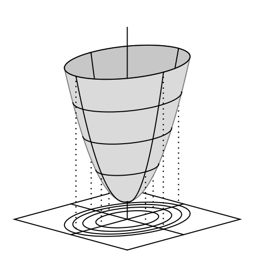
Figure 3 & 5 & 8: Combinations of "Plot" and "Graphics" using "Show". Axes and plot markers are all drawn manually.
Figure 4: Combination of "PolarPlot", "Graphics" and "Show", using equations developed in the text.
Figure 5: One dimensional curves in three dimensional space, another line drawing. Slightly different than Figure 2, in that the curve is given a thickness based on it's height along the view vector.
Figure 7: The Data Shot! As with 3/5/8, a combination of "Show", "Plot", and "Graphics", but worth mentioning on its own. Parameters for the cubic fit, in Table II, were computed using Bash, python, and gnuplot.
The last step is to export the images from inkscape into ".eps" format, the preferred format for ".tex" figures.
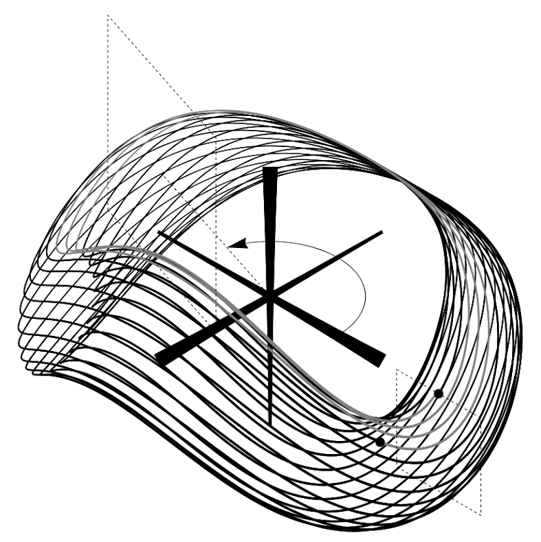
The much-improved version three is already submitted to another journal for consideration. In the meantime, I'm using the custom algorithms to draw torus figures associated with precession of two-dimensional oscillator orbits in an anharmonic potential:
$\dagger\dagger$ Brad $\dagger\dagger$
Edit: Challenges to the Reader
- Section IV.B.2 is confusing people. What is wrong here?
- Measurement challenges:
- Accurately and precisely measure the phase space trajectories by obtaining values (p,q) throughout time, in a minimal-friction experiment.
- Measure a large enough range of $K(\alpha)$ and distinguish between EllipticK and the Kidd-Fogg formula, by extracting polynomial fit parameters.


