WeightedAdjacencyMatrix and WeightedAdjacencyGraph are not consistent with each other. One uses 0 for non-existent edges, the other uses Infinity. What is the reasoning for this?

I reported this to support a long time ago, and I was told that it is by design. This question is to clarify why this is a desirable design.

Demonstration:

g = Graph[{1, 2, 3}, {1 <-> 2}, EdgeWeight -> {5.}]

WeightedAdjacencyMatrix[g] // Normal
(* {{0, 5., 0}, {5., 0, 0}, {0, 0, 0}} *)

As you can see, the element representing no connections is 0. But WeightedAdjacencyGraph just converts this to a weight

WeightedAdjacencyGraph@WeightedAdjacencyMatrix[g]

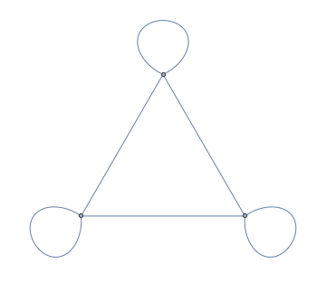
PropertyValue[%, EdgeWeight]
(* {0, 5., 0, 0, 0, 0} *)

This inconsistency usually causes inconvenience. What is its advantage?

Also, what is a performant and convenient way to work around this problem and cycle the graph through a weighted adjacency matrix representation?

Remember that people typically work with sparse graphs which may be large, often large enough that a dense adjacency matrix does not comfortably fit into memory. How do I then replace all the 0 entries in the sparse matrix with Infinity, while keeping the matrix sparse? This seems to be non-trivial, and is asked here:

• https://mathematica.stackexchange.com/questions/131834/directly-change-the-background-value-of-a-sparsearray

Thus a reliable way to cycle through a sparse matrix representation seems to be

WeightedAdjacencyGraph[
 With[{sa = WeightedAdjacencyMatrix[g]},
  SparseArray[Most@ArrayRules[sa], Dimensions[sa], Infinity]
  ],
 DirectedEdges -> DirectedGraphQ[g]
 ]

This is hardly convenient for such a common and simple operation.