Last week
Vi Hart submitted a new class titled
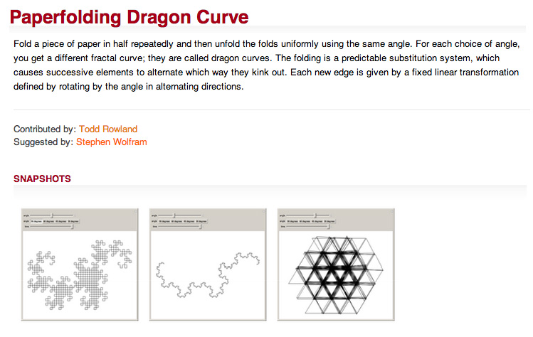
Doodling in Math Class: DRAGONS. There, she introduced a family of fractals known as
dragon curves, see here below the most famous one, the Heighway dragon:
The Heighway dragon (also known as the HarterHeighway dragon or the Jurassic Park dragon) was first investigated by NASA physicists John Heighway, Bruce Banks, and William Harter. It was described by Martin Gardner in his Scientific American column Mathematical Games in 1967. Many of its properties were first published by Chandler Davis and Donald Knuth. It appeared on the section title pages of the Michael Crichton novel Jurassic Park.
? Wikipedia
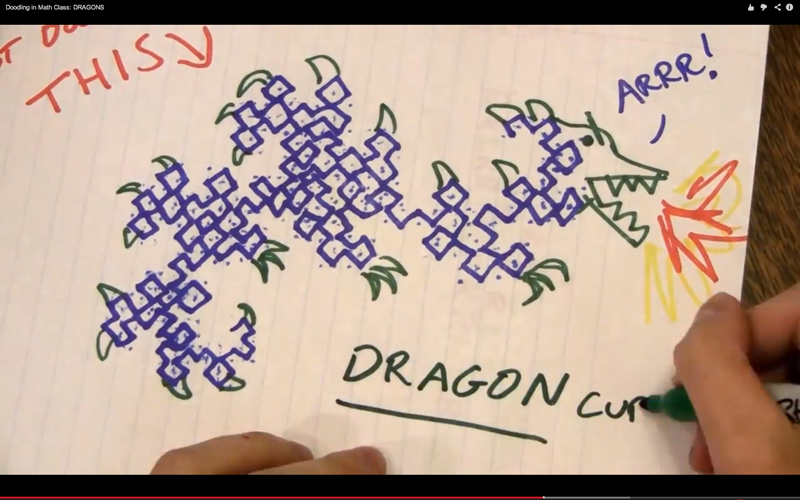
Wouldnt it be great to doodle fractals as fast as she does? What about doodling dragons in Mathematica?
Two years ago, when I was playing with the mind-blowing
Tree Bender demonstration by
Theodore Gray, I spotted a striking property. When the two branch-locators were placed in a symmetrical arrangement along the pair of horizontal line-segments {{-0.5,0.5},{0.5,0.5}} and {{-0.5,-0.5},{0.5,-0.5}}, the resulting trees were always forming dragons!
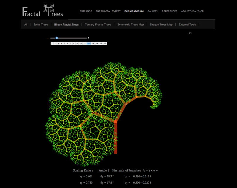
I was so excited by this observation that I ended up carrying out a whole
project about fractal trees, I published two papers presenting the n-ary symmetric trees with tip-to-tip self-contact, I 3D-printed some
SuperFractals generated by these trees, and I generalized this special class of fractals to three dimensional fractal trees during my participation at the 2013
Wolfram Science Summer School. For now lets focus on doodling dragons, I will talk about these related projects in future discussions.
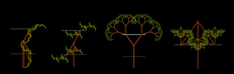
There are four different ways to place symmetrically the pair of locators along the pair of horizontal lines:
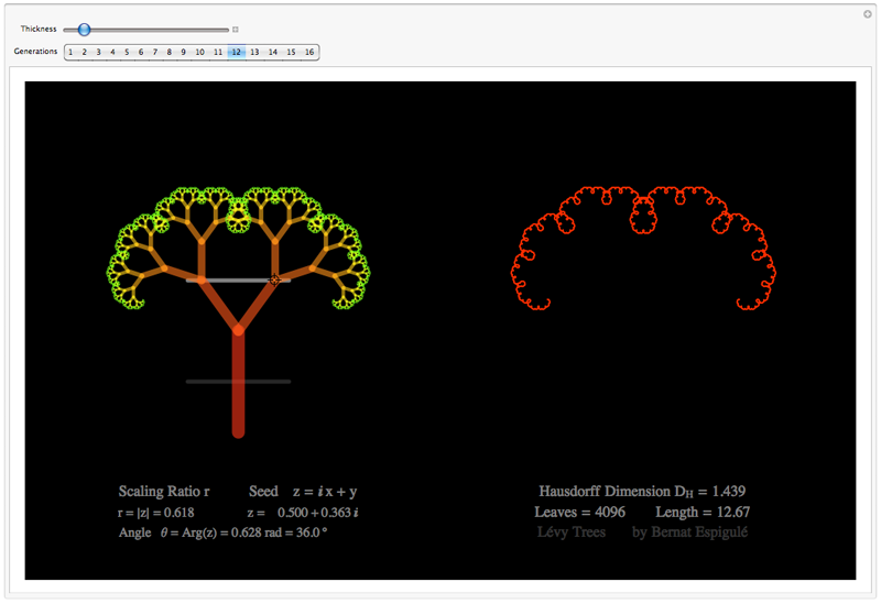
- One with the first pair of branches constrained to move along the upper line in a mirror symmetric way: Lévy Trees.
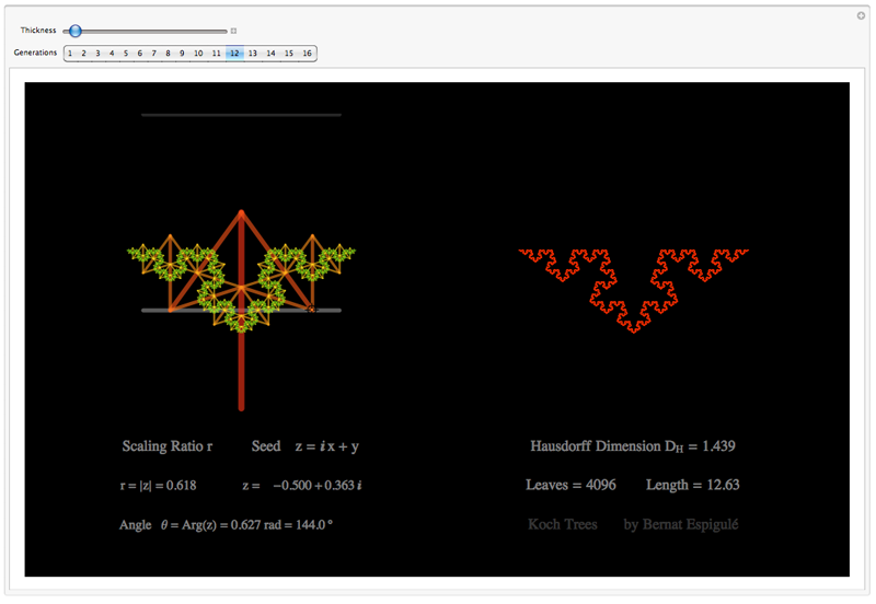
- One with the first pair of branches constrained to move along the lower line in a mirror symmetric way: Koch Trees.
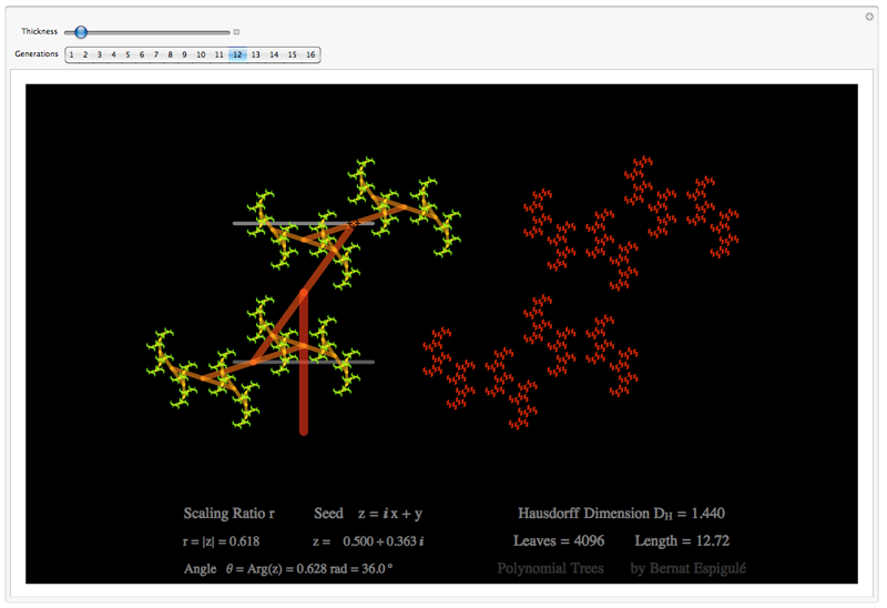
- One with the first pair of branches constrained to move along both horizontal lines in an opposite way to each other, 180º: Polynomial Trees.
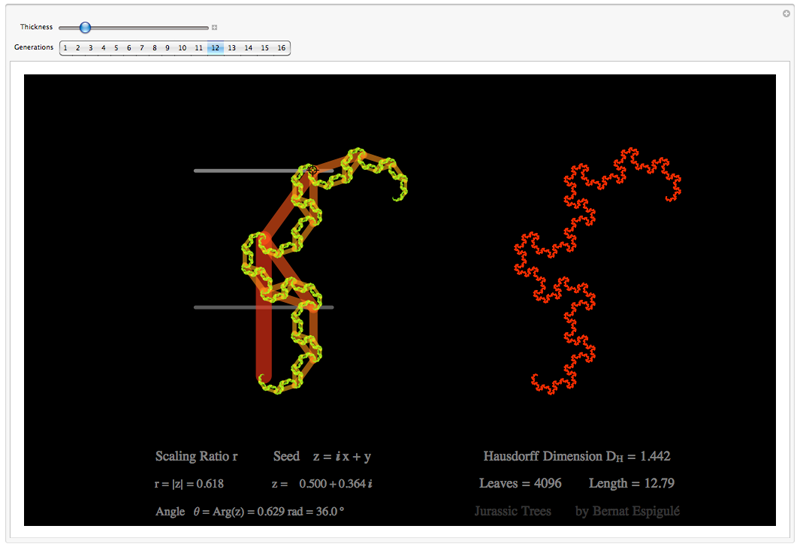
- And one with the first pair of branches constrained to move along both horizontal lines in a mirror symmetric way: Jurassic Park Trees.
Here below you have my pieces of code for doodling the four different kinds of binary dragon trees. Notice that Ive also added the final leaves in red and some meaningful labels to explore these trees with high precision (press Alt-key while moving the branch locator to slowly change the parameters).
Lévy Trees Doodler
Manipulate[
Module[{branches=NestList[Flatten[Map[{{#[[2]],#[[2]]+{Reverse[{pt1[[1]],0.5}],{-1,1}*{pt1[[1]],0.5}}.(#[[2]]-#[[1]])},{#[[2]],#[[2]]+{Reverse[{-pt1[[1]],0.5}],{-1,1}*{-pt1[[1]],0.5}}.(#[[2]]-#[[1]])}}&,#],1]&,{{{0,-1},{0,0}}},gen]},
Graphics[{
{CapForm["Round"],Gray,Thickness[0.005],Opacity[0.3],Line[{{-0.5,-0.5},{0.5,-0.5}}]},
{CapForm["Round"],Gray,Thickness[0.005],Line[{{-0.5,0.5},{0.5,0.5}}]},
{(*Tree*)MapIndexed[{Hue[0.022*#2[[1]],0.9,1,0.6],CapForm["Round"],Thickness[th*0.77^#2[[1]]],Line[#]}&,branches]},
{(*Leaves*)MapIndexed[{Hue[0.03(*gen*),1,1,0.9],CapForm["Round"],Thickness[th*0.82^(gen+1)],Translate[Line[#],{4,0}]}&,Drop[branches,gen]]},
(*Labels*)
{Inset[Style[Text@TraditionalForm@Style[Row[{"Scaling Ratio r"," "" "" Seed z = ",y+x*I}],18],Gray],{0,-1.6}]},
{Inset[Style[Text@TraditionalForm@Style[Row[{"r = |z|"," = ",SetAccuracy[Norm[{{pt1[[1]],0.5},{0,0}}],4]," ",z," = ",SetAccuracy[0.5,4]+SetAccuracy[pt1[[1]],4]I}],16],Gray],{0,-1.8}]},
{Inset[Style[Text@TraditionalForm@Style[Row[{"Angle \[Theta] = Arg(z)"," = ",SetAccuracy[VectorAngle[{pt1[[1]],0.5},{0,0.5}],4]," rad = ",SetAccuracy[180/Pi*VectorAngle[{pt1[[1]],0.5},{0,0.5}],2]"\[Degree] "}],16],Gray],{0,-2}]},
{Inset[Style[Text@TraditionalForm@Style[Row[{"Hausdorff Dimension \!\(\*SubscriptBox[\(D\), \(H\)]\) = ",SetAccuracy[ Log[2]/Log[1/Norm[{{pt1[[1]],0.5},{0,0}}]],4]}],18],Gray],{4.,-1.6}]},
{Inset[Style[Text@TraditionalForm@Style[Row[{"Leaves = ",Count[Drop[branches,gen],_Real,\[Infinity]]/4" "" ""Length = ",SetAccuracy[Count[Drop[branches,gen],_Real,\[Infinity]]/4*(Norm[{{pt1[[1]],0.5},{0,0}}]^gen),3]}],18],Gray],{4.,-1.8}]},
{Inset[Style[Text@TraditionalForm@Style[Row[{"Lévy Trees by Bernat Espigulé"}],18],Gray, Opacity[0.4]],{4.,-2}]}},
PlotRange->{{-2.1,6.1},{-2.1,2.1}},ImageSize->{1000,600},Background->Black]],
{{th,0.02,"Thickness"},0.005,0.185},
{{gen,12,"Generations"},Range[1,16], ControlType -> SetterBar},
{{pt1,{0.5,0.5}},{-0.5,0.5},{0.5,0.5},Locator}]
Koch Trees Doodler
Manipulate[
Module[{branches=NestList[Flatten[Map[{{#[[2]],#[[2]]+{Reverse[{pt1[[1]],-0.5}],{-1,1}*{pt1[[1]],-0.5}}.(#[[2]]-#[[1]])},{#[[2]],#[[2]]+{Reverse[{-pt1[[1]],-0.5}],{-1,1}*{-pt1[[1]],-0.5}}.(#[[2]]-#[[1]])}}&,#],1]&,{{{0,-1},{0,0}}},gen]},
Graphics[{{CapForm["Round"],Gray,Thickness[0.005],Opacity[0.7],Line[{{-0.5,-0.5},{0.5,-0.5}}]},{CapForm["Round"],Gray,Opacity[0.3],Thickness[0.005],Line[{{-0.5,0.5},{0.5,0.5}}]},
{(*FrTree*)MapIndexed[{Hue[0.022*#2[[1]],0.9,1,0.6],CapForm["Round"],Thickness[th*0.75^#2[[1]]],Line[#]}&,branches]},
{(*Red Leaves*)MapIndexed[{Hue[0.03(*gen*),1,1,0.9],CapForm["Round"],Thickness[th*0.84^(gen+1)],Translate[Line[#],{2,0}]}&,Drop[branches,gen]]},
(*Labels*)
{Inset[Style[Text@TraditionalForm@Style[Row[{"Scaling Ratio r"," "" "" Seed z = ",y+x*I}],18],Gray],{0,-1.2}]},
{Inset[Style[Text@TraditionalForm@Style[Row[{"r = |z|"," = ",SetAccuracy[Norm[{{pt1[[1]],0.5},{0,0}}],4]," ",z," = ",SetAccuracy[-0.5,4]+SetAccuracy[pt1[[1]],4]I}],16],Gray],{0,-1.4}]},
{Inset[Style[Text@TraditionalForm@Style[Row[{"Angle \[Theta] = Arg(z)"," = ",SetAccuracy[VectorAngle[{pt1[[1]],0.5},{0,0.5}],4]," rad = ",SetAccuracy[180/Pi*VectorAngle[{pt1[[1]],-0.5},{0,0.5}],2]"\[Degree] "}],16],Gray],{0,-1.6}]},
{Inset[Style[Text@TraditionalForm@Style[Row[{"Hausdorff Dimension \!\(\*SubscriptBox[\(D\), \(H\)]\) = ",SetAccuracy[ Log[2]/Log[1/Norm[{{pt1[[1]],0.5},{0,0}}]],4]}],18],Gray],{2.,-1.2}]},
{Inset[Style[Text@TraditionalForm@Style[Row[{"Leaves = ",Count[Drop[branches,gen],_Real,\[Infinity]]/4" "" ""Length = ",SetAccuracy[Count[Drop[branches,gen],_Real,\[Infinity]]/4*(Norm[{{pt1[[1]],0.5},{0,0}}]^gen),3]}],18],Gray],{2.,-1.4}]},
{Inset[Style[Text@TraditionalForm@Style[Row[{"Koch Trees by Bernat Espigulé"}],18],Gray, Opacity[0.4]],{2.,-1.6}]}},
PlotRange->{{-1.1,3.1},{-1.7,0.5}},ImageSize->{1000,600},Background->Black]],
{{th,0.01,"Thickness"},0.005,0.185},
{{gen,12,"Generations"},Range[1,16], ControlType -> SetterBar},
{{pt1,{0.5,0.5}},{-0.5,-0.5},{0.5,-0.5},Locator}]
Polynomial Trees Doodler
Manipulate[
Module[{branches=NestList[Flatten[Map[{{#[[2]],#[[2]]+{Reverse[{pt1[[1]],0.5}],{-1,1}*{pt1[[1]],0.5}}.(#[[2]]-#[[1]])},{#[[2]],#[[2]]+{Reverse[{-pt1[[1]],-0.5}],{-1,1}*{-pt1[[1]],-0.5}}.(#[[2]]-#[[1]])}}&,#],1]&,{{{0,-1},{0,0}}},gen]},
Graphics[{{CapForm["Round"],Gray,Thickness[0.005],Opacity[0.7],Line[{{-0.5,-0.5},{0.5,-0.5}}]},{CapForm["Round"],Gray,Thickness[0.005],Line[{{-0.5,0.5},{0.5,0.5}}]},
{(*FrTree*)MapIndexed[{Hue[0.022*#2[[1]],0.9,1,0.6],CapForm["Round"],Thickness[th*0.8^#2[[1]]],Line[#]}&,branches]},
{(*Red Leaves*)MapIndexed[{Hue[0.03(*gen*),1,1,0.9],CapForm["Round"],Thickness[th*0.84^(gen+1)],Translate[Line[#],{2,0}]}&,Drop[branches,gen]]},
(*Labels*)
{Inset[Style[Text@TraditionalForm@Style[Row[{"Scaling Ratio r"," "" "" Seed z = ",y+x*I}],18],Gray],{0,-1.6}]},
{Inset[Style[Text@TraditionalForm@Style[Row[{"r = |z|"," = ",SetAccuracy[Norm[{{pt1[[1]],0.5},{0,0}}],4]," ",z," = ",SetAccuracy[0.5,4]+SetAccuracy[pt1[[1]],4]I}],16],Gray],{0,-1.8}]},
{Inset[Style[Text@TraditionalForm@Style[Row[{"Angle \[Theta] = Arg(z)"," = ",SetAccuracy[VectorAngle[{pt1[[1]],0.5},{0,0.5}],4]," rad = ",SetAccuracy[180/Pi*VectorAngle[{pt1[[1]],0.5},{0,0.5}],2]"\[Degree] "}],16],Gray],{0,-2}]},
{Inset[Style[Text@TraditionalForm@Style[Row[{"Hausdorff Dimension \!\(\*SubscriptBox[\(D\), \(H\)]\) = ",SetAccuracy[ Log[2]/Log[1/Norm[{{pt1[[1]],0.5},{0,0}}]],4]}],18],Gray],{2.3,-1.6}]},
{Inset[Style[Text@TraditionalForm@Style[Row[{"Leaves = ",Count[Drop[branches,gen],_Real,\[Infinity]]/4" "" ""Length = ",SetAccuracy[Count[Drop[branches,gen],_Real,\[Infinity]]/4*(Norm[{{pt1[[1]],0.5},{0,0}}]^gen),3]}],18],Gray],{2.3,-1.8}]},
{Inset[Style[Text@TraditionalForm@Style[Row[{"Polynomial Trees by Bernat Espigulé"}],18],Gray, Opacity[0.4]],{2.3,-2}]}},
PlotRange->{{-1.7,3.7},{-2.1,1.5}},ImageSize->{1000,600},Background->Black]],
{{th,0.025,"Thickness"},0.005,0.185},
{{gen,12,"Generations"},Range[1,16], ControlType -> SetterBar},
{{pt1,{0.5,0.5}},{-0.5,0.5},{0.5,0.5},Locator}]
Jurassic Trees Doodler
Manipulate[
Module[{branches=NestList[Flatten[Map[{{#[[2]],#[[2]]+{Reverse[{pt1[[1]],0.5}],{-1,1}*{pt1[[1]],0.5}}.(#[[2]]-#[[1]])},{#[[2]],#[[2]]+{Reverse[{pt1[[1]],-0.5}],{-1,1}*{pt1[[1]],-0.5}}.(#[[2]]-#[[1]])}}&,#],1]&,{{{0,-1},{0,0}}},gen]},
Graphics[{{CapForm["Round"],Gray,Thickness[0.005],Opacity[0.7],Line[{{-0.5,-0.5},{0.5,-0.5}}]},{CapForm["Round"],Gray,Thickness[0.005],Line[{{-0.5,0.5},{0.5,0.5}}]},
{(*FrTree*)MapIndexed[{Hue[0.022*#2[[1]],0.9,1,0.6],CapForm["Round"],Thickness[th*0.72^#2[[1]]],Line[#]}&,branches]},
{(*Red Leaves*)MapIndexed[{Hue[0.03(*gen*),1,1,0.9],CapForm["Round"],Thickness[th*0.8^(gen+1)],Translate[Line[#],{2,0}]}&,Drop[branches,gen]]},
(*Labels*)
{Inset[Style[Text@TraditionalForm@Style[Row[{"Scaling Ratio r"," "" "" Seed z = ",y+x*I}],18],Gray],{0,-1.6}]},
{Inset[Style[Text@TraditionalForm@Style[Row[{"r = |z|"," = ",SetAccuracy[Norm[{{pt1[[1]],0.5},{0,0}}],4]," ",z," = ",SetAccuracy[0.5,4]+SetAccuracy[pt1[[1]],4]I}],16],Gray],{0,-1.8}]},
{Inset[Style[Text@TraditionalForm@Style[Row[{"Angle \[Theta] = Arg(z)"," = ",SetAccuracy[VectorAngle[{pt1[[1]],0.5},{0,0.5}],4]," rad = ",SetAccuracy[180/Pi*VectorAngle[{pt1[[1]],0.5},{0,0.5}],2]"\[Degree] "}],16],Gray],{0,-2}]},
{Inset[Style[Text@TraditionalForm@Style[Row[{"Hausdorff Dimension \!\(\*SubscriptBox[\(D\), \(H\)]\) = ",SetAccuracy[ Log[2]/Log[1/Norm[{{pt1[[1]],0.5},{0,0}}]],4]}],18],Gray],{2.3,-1.6}]},
{Inset[Style[Text@TraditionalForm@Style[Row[{"Leaves = ",Count[Drop[branches,gen],_Real,\[Infinity]]/4" "" ""Length = ",SetAccuracy[Count[Drop[branches,gen],_Real,\[Infinity]]/4*(Norm[{{pt1[[1]],0.5},{0,0}}]^gen),3]}],18],Gray],{2.3,-1.8}]},
{Inset[Style[Text@TraditionalForm@Style[Row[{"Jurassic Trees by Bernat Espigulé"}],18],Gray, Opacity[0.4]],{2.3,-2}]}},
PlotRange->{{-1.7,3.7},{-2.1,1.2}},ImageSize->{1000,600},Background->Black]],
{{th,0.03,"Thickness"},0.005,0.185},
{{gen,12,"Generations"},Range[1,16], ControlType -> SetterBar},
{{pt1,{0.5,0.5}},{-0.5,0.5},{0.5,0.5},Locator}]
As far as I know these four families of fractal trees have not been presented before so Ive just uploaded them on a single CDF to the Demonstration Project. I will share with you its url when published.
If you would like to explore other demonstrations dealing with these
dragons here are the links to the
Paperfolding Dragon Curve by
Todd Rowland, the
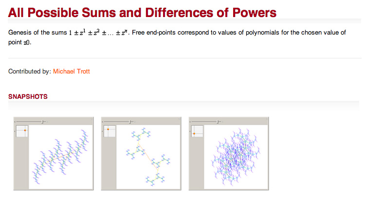
original Polynomial Trees by
Michael Trott (check also his recent posts (
1,
2,
3) about other creative ways of doodling in Mathematica ), and the classic
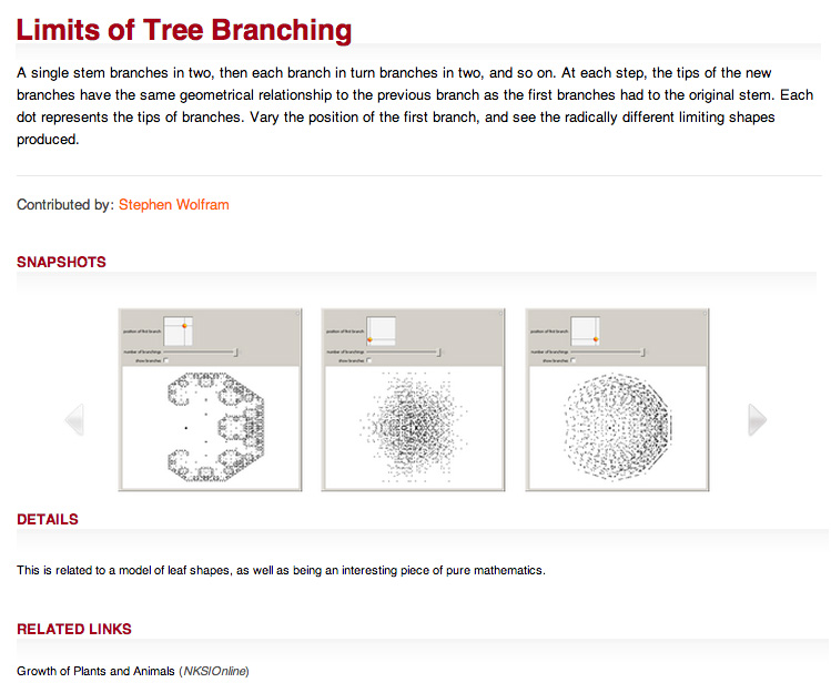
Limits of Tree Branching by
Stephen Wolfram.
Finally, if you liked
Theodore Grays Tree Bender, here you will find
my adapted CDF for exploring binary trees with color and with meaningful parameters to describe them precisely.
Thats all for today! Enjoy, and let me know if you had been lucky enough to find
a tree worthy of worship ;-).


