This was my approach.
Import data:
data = Import["C:\\Users\\bgood_000\\Downloads\\T0027.csv"];
and then examine (David Keith's answer above does this much better)
In[42]:= data[[1 ;; 100]]

Out[42]= {{"Model", "DPO2002B"}, {"Firmware Version",
  1.52}, {""}, {"Point Format", "Y", "", "", ""}, {"Horizontal Units",
   "S", "", "", ""}, {"Horizontal Scale", 4, "", "",
  ""}, {"Sample Interval", 0.00768049, "", "",
  ""}, {"Filter Frequency", 7.*10^7, "", "", ""}, {"Record Length",
  5189, "", "", ""}, {"Gating", "0.0% to 100.0%", "",
  "0.0% to 100.0%", ""}, {"Probe Attenuation", 10, "", 10,
  ""}, {"Vertical Units", "V", "", "V", ""}, {"Vertical Offset", 0,
  "", 0, ""}, {"Vertical Scale", 10, "", 2, ""}, {"Label", "", "", "",
   ""}, {"TIME", "CH1", "CH1 Peak Detect", "CH2",
  "CH2 Peak Detect"}, {-20., -7.4, -7.8,
  0.04, -0.12}, {-19.992, -7.4, -7, -0.04,
  0.12}, {-19.985, -7.4, -7.8, -0.04, -0.2}, {-19.977, -7.4, -7, \
-0.12, 0.04}, {-19.969, -7.4, -7.8, -0.12, -0.28}, {-19.962, -7.4, \
-7, -0.2, -0.04}, {-19.954, -7.4, -7.8, -0.2, -0.36}, {-19.946, -7.4, \
-6.6, -0.2, -0.12}, {-19.939, -7.4, -7.8, -0.2, -0.44}, {-19.931, \
-7.4, -6.6, -0.28, -0.2}, {-19.923, -7.4, -7.8, -0.36, -0.52}, \
{-19.916, -7, -6.6, -0.36, -0.28}, {-19.908, -7, -7.4, -0.44, -0.6}, \
{-19.9, -6.6, -6.2, -0.44, -0.28}, {-19.892, -7, -7.4, -0.44, -0.6}, \
{-19.885, -6.6, -6.2, -0.52, -0.36}, {-19.877, -6.6, -7, -0.52, \
-0.68}, {-19.869, -6.6, -5.8, -0.52, -0.44}, {-19.862, -6.2, -6.6, \
-0.6, -0.76}, {-19.854, -5.8, -5.4, -0.6, -0.52}, {-19.846, -5.8, \
-6.2, -0.6, -0.84}, {-19.839, -5.8, -5, -0.6, -0.6}, {-19.831, -5.4, \
-5.8, -0.68, -0.84}, {-19.823, -5, -4.6, -0.76, -0.6}, {-19.816, -5, \
-5.4, -0.76, -0.92}, {-19.808, -4.6, -4.2, -0.84, -0.68}, {-19.8, \
-4.6, -5, -0.84, -0.92}, {-19.793, -4.2, -3.4, -0.84, -0.76}, \
{-19.785, -3.8, -4.6, -0.84, -1}, {-19.777, -3.8, -3, -0.92, -0.76}, \
{-19.77, -3.4, -3.8, -0.92, -1}, {-19.762, -3, -2.2, -0.92, -0.84}, \
{-19.754, -2.6, -3.4, -0.92, -1.08}, {-19.747, -2.6, -1.8, -1, \
-0.84}, {-19.739, -2.2, -2.6, -1, -1.08}, {-19.731, -2.2, -1, -1, \
-0.84}, {-19.724, -1.4, -2.2, -1, -1.08}, {-19.716, -1.4, -0.6, -1, \
-0.84}, {-19.708, -1, -1.4, -1, -1.08}, {-19.7, -0.6,
  0.2, -0.92, -0.92}, {-19.693, -0.2, -1, -1, -1.08}, {-19.685, -0.2,
  1, -1, -0.84}, {-19.677, 0.2, -0.2, -0.92, -1.08}, {-19.67, 0.6,
  1.4, -1, -0.84}, {-19.662, 1, 0.2, -0.92, -1.08}, {-19.654, 1,
  2.2, -0.92, -0.84}, {-19.647, 1.8, 1, -0.92, -1}, {-19.639, 1.8,
  2.6, -0.92, -0.84}, {-19.631, 2.2, 1.4, -0.84, -1}, {-19.624, 2.2,
  3, -0.92, -0.76}, {-19.616, 2.6, 2.2, -0.84, -0.92}, {-19.608, 3,
  3.8, -0.84, -0.76}, {-19.601, 3, 2.6, -0.76, -0.92}, {-19.593, 3.4,
  4.2, -0.76, -0.68}, {-19.585, 3.8, 3, -0.76, -0.84}, {-19.578, 3.8,
  4.6, -0.76, -0.6}, {-19.57, 4.2, 3.4, -0.68, -0.84}, {-19.562, 4.2,
  5, -0.76, -0.52}, {-19.555, 4.6, 4.2, -0.68, -0.76}, {-19.547, 5,
  5.4, -0.6, -0.52}, {-19.539, 5.4, 4.6, -0.52, -0.68}, {-19.531, 5.4,
   6.2, -0.52, -0.44}, {-19.524, 5.4, 5, -0.52, -0.6}, {-19.516, 5.4,
  6.2, -0.52, -0.36}, {-19.508, 5.8, 5.4, -0.44, -0.52}, {-19.501,
  6.2, 6.6, -0.44, -0.28}, {-19.493, 6.2,
  5.8, -0.36, -0.52}, {-19.485, 6.2, 7, -0.36, -0.2}, {-19.478, 6.6,
  5.8, -0.28, -0.44}, {-19.47, 6.6, 7.4, -0.28, -0.2}, {-19.462, 7,
  6.2, -0.28, -0.36}, {-19.455, 7, 7.4, -0.28, -0.12}, {-19.447, 7,
  6.6, -0.2, -0.28}, {-19.439, 7.4, 7.8, -0.2, -0.04}, {-19.432, 7.4,
  6.6, -0.12, -0.2}, {-19.424, 7.4, 7.8, -0.12, 0.04}, {-19.416, 7.4,
  6.6, -0.04, -0.12}, {-19.409, 7.4, 7.8, -0.04, 0.12}, {-19.401, 7.4,
   7, 0.04, -0.04}, {-19.393, 7.4, 7.8, 0.04, 0.2}, {-19.386, 7.4, 7,
  0.12, -0.04}, {-19.378, 7.4, 7.8, 0.12, 0.28}, {-19.37, 7.4, 6.6,
  0.12, 0.04}, {-19.363, 7.4, 7.8, 0.12, 0.28}}
So there's a header in position 16
In[48]:= data[[16]]

Out[48]= {"TIME", "CH1", "CH1 Peak Detect", "CH2", "CH2 Peak Detect"}
For some reason the last element is empty so I'll pick out everything after the header up to the penultimate element.
In[77]:= plotData = data[[17 ;; -2]];
From the header I know the positions of time and voltages (CH1, CH2)
In[94]:= time = plotData[[All, 1]];
ch1 = plotData[[All, 2]];
ch2 = plotData[[All, 4]];
Thread the timebase into each extracted channel amplitude list.
dataset1 = Thread[{time, ch1}];
dataset2 = Thread[{time, ch2}];
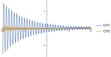
And plot
In[99]:= ListLinePlot[{
  dataset1, dataset2
  },
 PlotRange -> All,
 PlotLegends -> {"CH1", "CH2"}
 ]
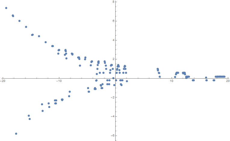
We can obtain a coarse fit of CH1 by first looking at the peaks
ListPlot[
 FindPeaks[TimeSeriesResample[TimeSeries[dataset1]]],
 PlotRange -> Full
 ]
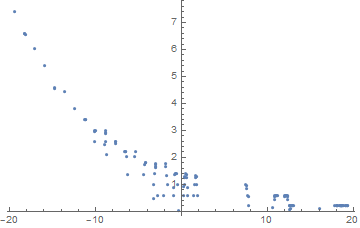
Lets extract the upper component of the signal
fittingData = FindPeaks[TimeSeriesResample[TimeSeries[dataset1]]];
upper = Select[fittingData["Path"], #[[2]] > 0 &];
And examine
ListPlot[upper, Joined -> False]
Find a nonlinear model for the data,
$$a \exp{(-bx)} $$ is a good start
nlm = NonlinearModelFit[upper, a*Exp[-b*x], {a, b}, x];
Check nlm and show atop the original plot
Show[{
  Plot[nlm[x], {x, -20, 20}, PlotStyle -> {Dashed, Thick, Blue},
   PlotLegends -> nlm],
  ListLinePlot[{
    dataset1, dataset2
    },
   PlotRange -> All,
   PlotLegends -> {"CH1", "CH2"}
   ]
  }, PlotRange -> All]
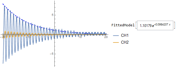
Repeat for CH2 and refine model if necessary.
Best Regards,
Ben


