In my previous post GraphImage2List, I created the tool that changes graph-image-data to numeric-data in order to do a Machine Learning using graph-image-data. However, it can't deal with multi-colored graph-image-data. So I create a new tool by ImageGraphics function. ImageGraphics is one of my favorite new functions in Wolfram Language 11.1.
Goal
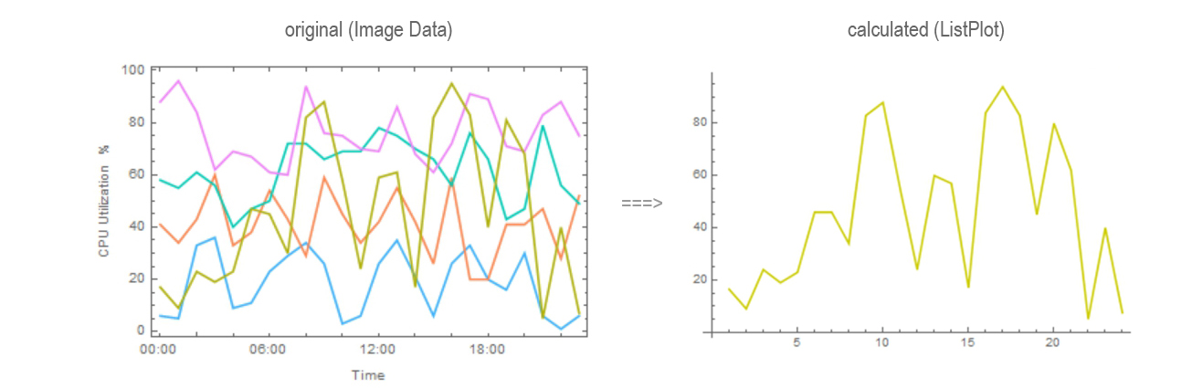
The left is the original graph(image data) like CPU Utilization of five virtual machines. The right is the graph(ListPlot) of yellow-green line picked up by the new tool.
The tool comes in three steps.
Step 1
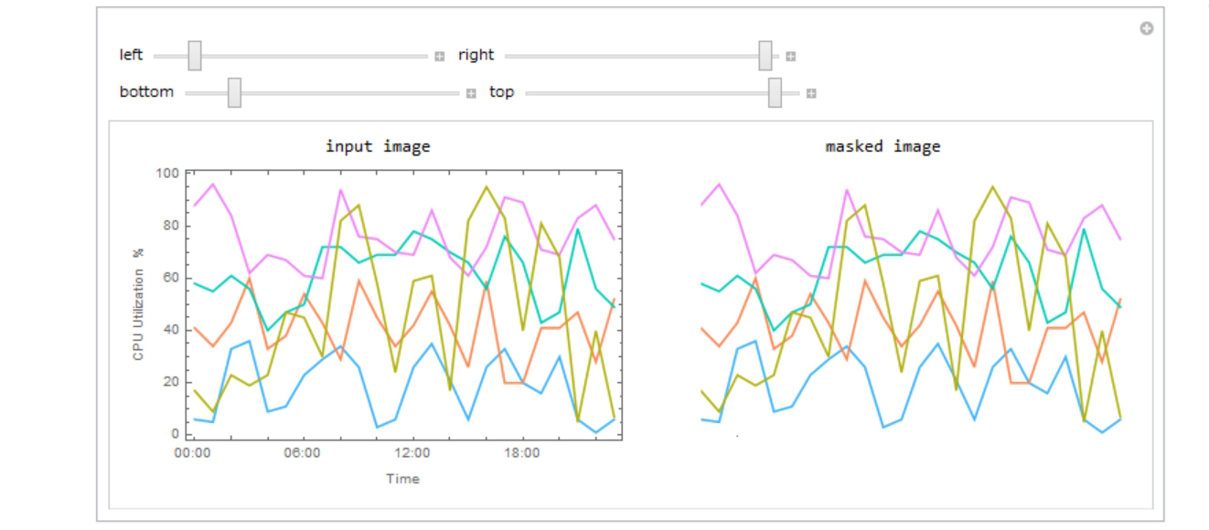
In the first step, My MakeMasking function masks unnecessary areas around the original image data like plot label, frame and ticks. It outputs "maskedimage".
MakeMasking[img_] := Module[{},
  size = {sizex, sizey} = ImageDimensions[img];
  backimg = Image[Table[1, {sizey}, {sizex}]];
  Manipulate[
   Grid[{{"input image", "masked image"},
     {Show[img, ImageSize -> size],
      Show[
       maskedimg =
        ImageCompose[backimg,
         ImageTrim[
          img, {{left, bottom}, {right, top}}], {left + right,
           bottom + top}/2], ImageSize -> size]}}],
   Row[{Control[{left, 0, sizex, 1}],
     Control[{{right, sizex}, 0, sizex, 1}]}, "   "],
   Row[{Control[{bottom, 0, sizey, 1}],
     Control[{{top, sizey}, 0, sizey, 1}]}, "   "]
   ]
  ]
The left is the original. The right is masked image.
Step 2
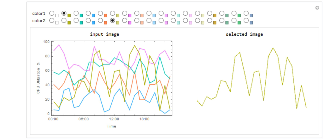
In this step, My SelectColors function selects the areas of two near colors in ImageGraphics output of "maskedimage". ImageGraphics function returns the content of image. The colors are below.
maskedimggraphics = ImageGraphics[maskedimg, PlotRangePadding -> None];
maskedimggraphics[[1, 2, #, 1]] & /@ Range[Length[maskedimggraphics[[1, 2]]]]

My SelectColors function uses the content and outputs the selected area as "selectpts".
SelectColors[img_, maskedimggraphics_] := Module[{},
  {sizex, sizey} = size = ImageDimensions[img] // N;
  frame = {{0., 0.}, {0., sizey}, {sizex, sizey}, {sizex, 0.}};
  l = Length[maskedimggraphics[[1, 1]]];
  colors =
   maskedimggraphics[[1, 2, #, 1]] & /@
    Range[Length[maskedimggraphics[[1, 2]]]];
  Manipulate[
   Grid[{{"input image", "selected image"},
     {Show[img, ImageSize -> ImageDimensions[img]],
      Graphics[
       GraphicsComplex[Join[maskedimggraphics[[1, 1]], frame],
        Join[{LABColor[
          0.9988949153893414, -3.6790844387894895`*^-6,
           0.00042430735605277474`],
          FilledCurve[{{Line[{l + 1, l + 2, l + 3, l + 4}]}}]},
         selectpts =
          FirstCase[maskedimggraphics[[1, 2]], {#, ___},
             Nothing] & /@ {color1, color2}]],
       ImageSize -> size]}}], {{color1, colors[[2]]}, colors,
    ControlType -> RadioButton,
    Method -> "Queued"}, {{color2, colors[[2]]}, colors,
    ControlType -> RadioButton, Method -> "Queued"},
   SynchronousUpdating -> False]
  ]
The left is the original. The right is selected image.
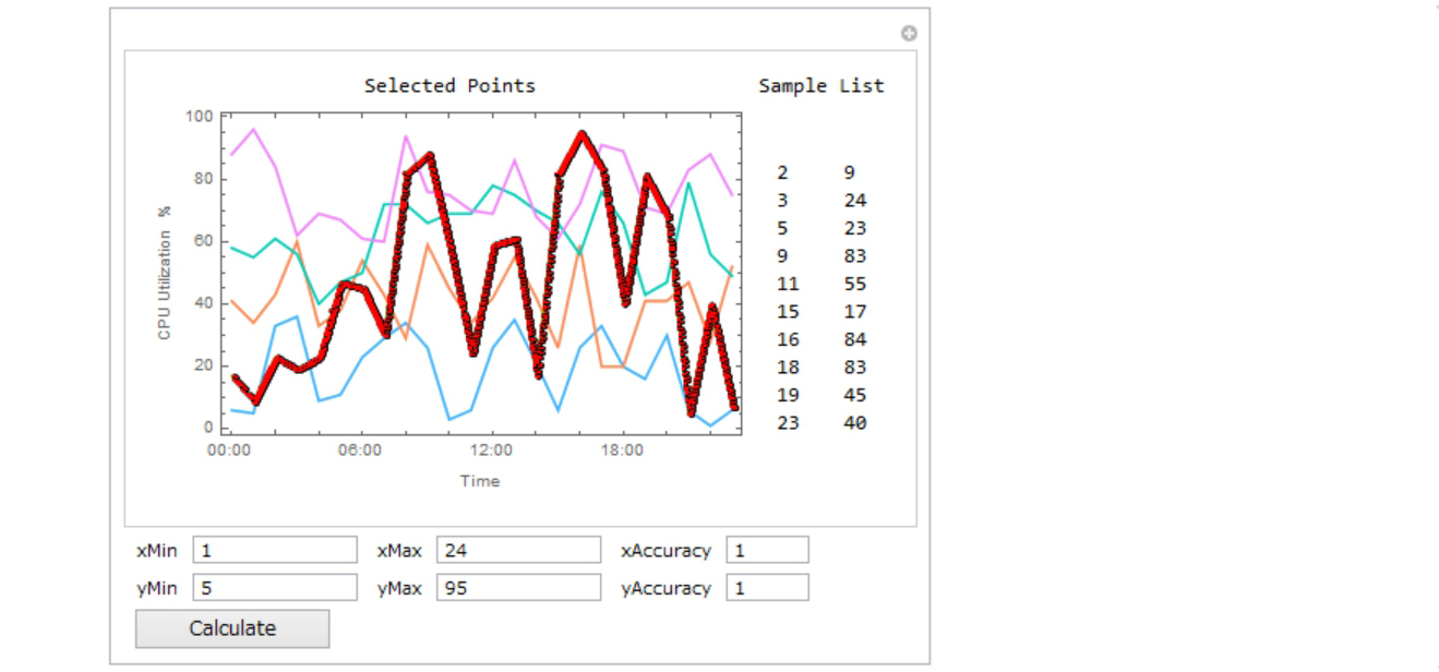
Step 3
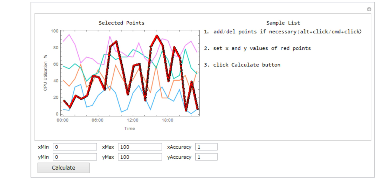
You can make list in the next process by using my GetList2 function.
1. Add/del points with alt+click(WINDOWS)/cmd+click(MAC) if necessary
2. Set x and y values(Min, Max, Accuracy) of red points
3. Click Calculate button
GetList2[img_, imggraphics_, selectpts_] := Module[{},
  ClearAll[list]; list = {};
  Manipulate[
   Grid[{{"Selected Points", "Sample List"},
     {Show[img, Graphics[{Point[u]}],
       ImageSize -> ImageDimensions[img]],
      Dynamic[If[(ValueQ[list] == False) || (list == {}),
        "1? add/del points if necessary(alt+click/cmd+click?\n
        2. set x and y values of red points\n
        3. click Calculate button",
        Sort[RandomSample[list, UpTo[10]]] // TableForm]]}},
    Alignment -> Top],
   Row[{Control[{xMin, {0}, InputField, ImageSize -> 100}],
     Control[{xMax, {100}, InputField, ImageSize -> 100}],
     Control[{{xAccuracy, 1}, InputField, ImageSize -> 50}]}, "    "],
   Row[{Control[{yMin, {0}, InputField, ImageSize -> 100}],
     Control[{yMax, {100}, InputField, ImageSize -> 100}],
     Control[{{yAccuracy, 1}, InputField, ImageSize -> 50}]}, "    "],
   Row[{Button["Calculate",
      list = locator2coordinate2[u, xMin, xMax, xAccuracy, yMin, yMax,
          yAccuracy];, ImageSize -> 120, Method -> "Queued"]}, "  "],
   {{u, Sort[GetPointsfromImageGraphics[imggraphics, selectpts]]},
    Locator, LocatorAutoCreate -> True,
    Appearance -> Style["\[FilledCircle]", Red, 3]},
   ControlPlacement -> {Bottom, Bottom, Bottom},
   SynchronousUpdating -> False]
  ]

locator2coordinate2[points_, xMin_, xMax_, xAccuracy_, yMin_, yMax_,
  yAccuracy_] :=
 Module[{solvex, solvey, pointsx, pointsy, points2, coordinatesL,
   coordinatesH, nearx, nearxpos, tmp},
  solvex =
   Solve[{a*#[[1]] + b == xMin, a*#[[2]] + b == xMax}, {a, b}] &@
    MinMax[points[[All, 1]]];
  pointsx = Flatten[({a, b} /. solvex).{#, 1} & /@ points[[All, 1]]];
  solvey =
   Solve[{c*#[[1]] + d == yMin, c*#[[2]] + d == yMax}, {c, d}] &@
    MinMax[points[[All, 2]]];
  pointsy = Flatten[({c, d} /. solvey).{#, 1} & /@ points[[All, 2]]];
  points2 = Sort[Thread[{pointsx, pointsy}]];
  coordinatesL = (points2 //. {s___, {u_, v_}, {u_, w_},
       t___} -> {s, {u, v}, t});
  coordinatesH = (points2 //. {s___, {u_, v_}, {u_, w_},
       t___} -> {s, {u, w}, t});
  (* High value *)
  nearx = (Nearest[coordinatesH[[All, 1]], #, 1] & /@
      Range[xMin, xMax, xAccuracy] // Flatten);
  nearxpos =
   Position[coordinatesH[[All, 1]], #, 1, 1] & /@ nearx // Flatten;
  nearyH = Round[#, yAccuracy] & /@ coordinatesH[[All, 2]][[nearxpos]];
  (* Low value *)
  nearx = (Nearest[coordinatesL[[All, 1]], #, 1] & /@
      Range[xMin, xMax, xAccuracy] // Flatten);
  nearxpos =
   Position[coordinatesL[[All, 1]], #, 1, 1] & /@ nearx // Flatten;
  nearyL = Round[#, yAccuracy] & /@ coordinatesL[[All, 2]][[nearxpos]];
  (* Middle value *)
  nearyM = (nearyH + nearyL)/2;
  (* Combination value *)
  tmp = ((#[[1]] + #[[3]])/2) & /@ Partition[nearyM, 3, 1];
  nearyC = Table[Which[
     nearyM[[i + 1]] > tmp[[i]], nearyH[[i + 1]],
     nearyM[[i + 1]] < tmp[[i]], nearyL[[i + 1]],
     True, Round[nearyM[[i + 1]], yAccuracy]], {i, Length[tmp]}];
  PrependTo[nearyC, Round[nearyM[[1]], yAccuracy]];
  AppendTo[nearyC, Round[nearyM[[-1]], yAccuracy]];
  Thread[{Range[xMin, xMax, xAccuracy], nearyC}]
  ]
Set x and y values(Min, Max, Accuracy) of red points and click.
Then it outputs "list".
list

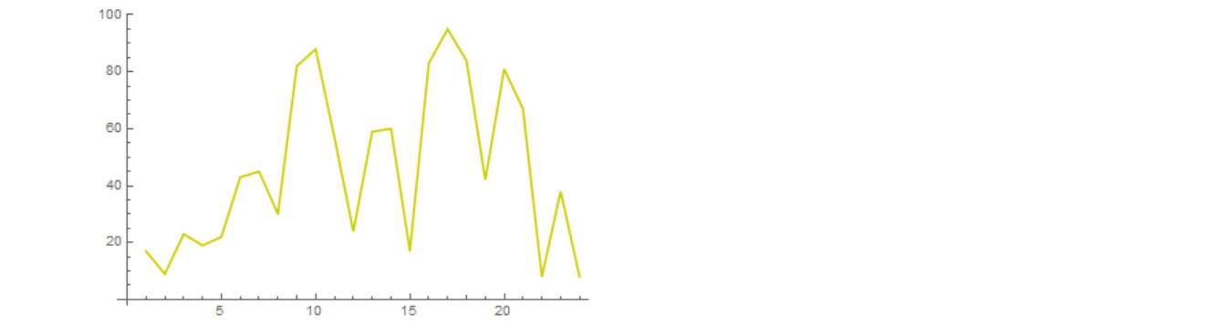
ListPlot of the list is below.
ListPlot[Style[list, RGBColor[204/255, 204/255, 0]], Joined -> True]
Differences
When GetList2 converts area selected in Step 2. to coordinates, there are some points of the same x coordinate. So my locator2coordinate2 function outputs 4 lists of y coordinate, high, low, middle and combination as nearyH, nearyL, nearyM and nearyC. As I show below, nearyC seems to be better than others.
I create this image data below.
data = {{6, 5, 33, 36, 9, 11, 23, 29, 34, 26, 3, 6, 26, 35, 21, 6, 26, 33, 20, 16, 30, 6, 1, 6},
   {41, 34, 43, 60, 33, 38, 54, 43, 29, 59, 45, 34, 42, 55, 42, 26, 59, 20, 20, 41, 41, 47, 28, 52},
   {58, 55, 61, 56, 40, 47, 50, 72, 72, 66, 69, 69, 78, 75, 70, 66, 56, 76, 66, 43, 47, 79, 56, 49},
   {88, 96, 84, 62, 69, 67, 61, 60, 94, 76, 75, 70, 69, 86, 68, 61, 72, 91, 89, 71, 69, 83, 88, 75},
   {17, 9, 23, 19, 23, 47, 45, 30, 82, 88, 58, 24, 59, 61, 17, 82, 95, 83, 40, 81,  68, 5, 40, 7}};
graph =
   DateListPlot[data, {2017, 5, 20, 0}, Frame -> True,
   FrameLabel -> {"Time", "CPU Utilization %"}, PlotStyle -> 96];
img = Rasterize[graph]
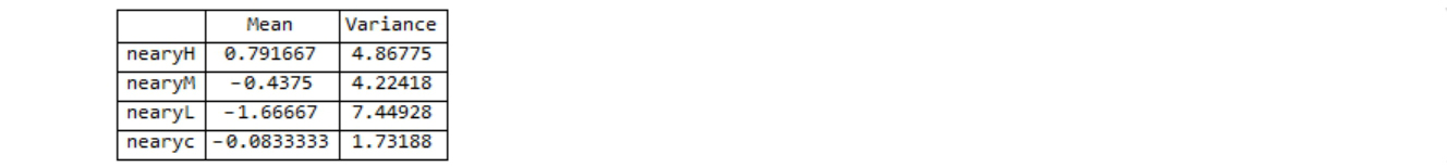
Mean and Variance of the difference between the true list(data) and calculated 4 list(nearyH, nearyL, nearyM and nearyC) are below and nearyC is the best of all.
Grid[
 Join[{{"", "nearyH", "nearyM", "nearyL", "nearyc"}},
   Join[{{"Mean", "Variance"}},
         {Mean[#], Variance[#]} & /@ {nearyH - #, nearyM - #, nearyL - #,
          nearyC - #} &@data[[5]] // N] // Transpose] // Transpose,
 Frame -> All]
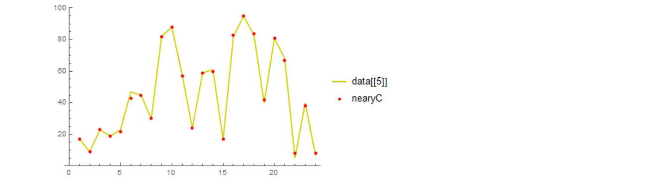
ListPlot[{Legended[Style[data[[5]], RGBColor[204/255, 204/255, 0]],
   "data[[5]]"], Legended[Style[nearyC, Red], "nearyC"]},
   Joined -> {True, False}, PlotRange -> {0, 100}]
 Attachments:


