Shadow mapping is a process of applying shadows to a computer graphic. Graphics3D allows the user to specify lighting conditions for the surfaces of 3D graphical primitives, however, visualising the shadow an object projects onto a surface requires the processes of shadow mapping. Each pixel of the projection surface must check if it is visible from the light source; if this check returns false then the pixel forms a shadow. This becomes a problem of geometric intersections, i.e., for this case, the intersection between a line and a triangle. For a 3D model with 100s and more of polygons, repeated intersection tests across the entire model for each pixel is an extremely costly (and inefficient) task. Now this becomes a problem of search optimisation.

Obtaining Data

This project uses 3D models from SketchUp's online repository which are converted to COLLADA files using SketchUp. The functions used are held in a package, accessible via github along with all the data referenced throughout.

(* load package and 3D model *)
<< "https://raw.githubusercontent.com/b-goodman/\
GeometricIntersections3D/master/GeometricIntersections3D.wl";

modelPath = 
  "https://raw.githubusercontent.com/b-goodman/\
GeometricIntersections3D/master/Demo/House/houseModel4.dae";

(* vertices of model's polygons *)
polyPoints = Delete[0]@Import[modelPath, "PolygonObjects"];

(* import model as region *)
modelRegion = Import[modelPath, "MeshRegion"];

(* use region to generate minimal bounding volume *)
cuboidPartition = Delete[0]@BoundingRegion[modelRegion, "MinCuboid"];

(* verify *)
Graphics3D[{
  Polygon[polyPoints],
  {Hue[0, 0, 0, 0], EdgeForm[Black], Cuboid[cuboidPartition]}
  }, Boxed -> False]

Generate a Bounding Volume Hierarchy (BVH)

Shadow mapping (and more generally collision testing) may be optimised via space partitioning achieved by dividing the 3D model's space into a hierarchy of bounding volumes (BV) stored as a graph, thus forming a bounding volume hierarchy. The simplest case uses the result of an intersection between a ray and a single BV for the entire model to discard all rays which don't come close to any of the model's polygons. Of course, those which do pass the first test must still be tested against the entire model so the initial BV is subdivided with each sub BV assigned to a particular part of the model hence reducing the total amount of polygons to be tested against. The initial BV forms the root of the tree and it's subdivisions (leaf boxes) are joined via edges. We can add more levels to the tree by repeating the subdivision for each of the leaf boxes and ultimately refining the search for potential intersecting polygons.

(* Begin tree.  Initial AABB is root.  Subdivide root AABB and link returns to root *) 
newBVH[cuboidPartitions_,polyPoints_]:=Block[{
newLevel,edges
},
newLevel=Quiet[cullIntersectingPartitions[cuboidSubdivide[cuboidPartitions],polyPoints]];
edges=cuboidPartitions\[DirectedEdge]#&/@newLevel;
Return[<|
"Tree"->TreeGraph[edges],
"PolygonObjects"->polyPoints
|>];
];

bvh = newBVH[{cuboidPartition}, polyPoints];

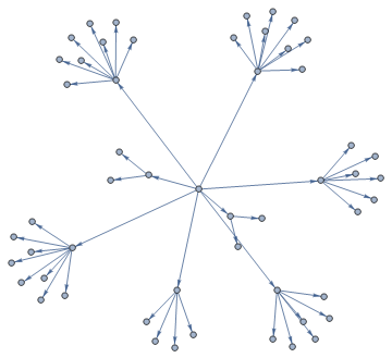
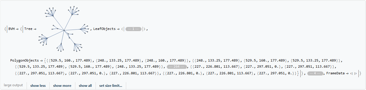
The BVH is a tree graph with the model's polygon vertices encapsulated within an association

Keys[bvh]

{"Tree", "PolygonObjects"}

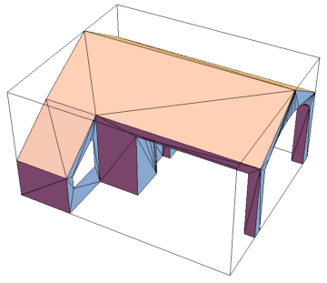
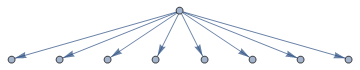
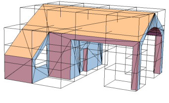
The BVH consists of a root box derived from the model's minimal bounding volume and it's 8 sub-divisions

bvh["Tree"]

The boxes at the lowest level of the BVH are the leaf boxes

leafBoxesLV1 = 
  Select[VertexList[bvh["Tree"]], 
   VertexOutDegree[bvh["Tree"], #] == 0 &];

Graphics3D[{
  Polygon[polyPoints],
  {Hue[0, 0, 0, 0], EdgeForm[Black], Cuboid /@ leafBoxesLV1}
  }, Boxed -> False]

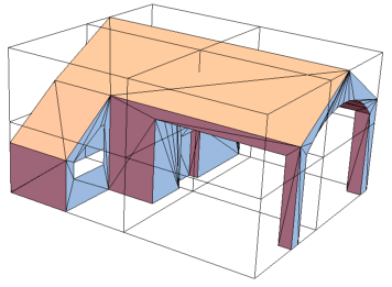
Adding a new level sub-divides each leaf box into 8 sub-divisions.

With[{
  testCuboid = {{0, 0, 0}, {10, 10, 10}}
  },
 Manipulate[
  Graphics3D[{
    If[n == 0, Cuboid[testCuboid], 
     Cuboid /@ Nest[cuboidSubdivide, testCuboid, n]]
    }, Boxed -> False, Axes -> {True, False}],
  {{n, 0}, 0, 4, 1}
  ]
 ]

The time needed for each addition to the BVH increases dramatically.

Length /@ NestList[cuboidSubdivide, {{{0, 0, 0}, {1, 1, 1}}}, 5]

 {1, 8, 64, 512, 4096, 32768}

1-2 added levels is usually enough for the models used in this project.

(* Each new subdivision acts as root.  For each, subdivide further and remove any non-intersecting boxes.  Link back to parent box as directed edge *)
addLevelBVH[BVH_]:=Block[{
tree=BVH["Tree"],polyPoints=BVH["PolygonObjects"],returnEdges
},
Module[{
subEdges=Map[
Function[{levelComponent},levelComponent\[DirectedEdge]#&/@Quiet@cullIntersectingPartitions[cuboidSubdivide[levelComponent],polyPoints]],
Pick[VertexList[tree],VertexOutDegree[tree],0]]
},
returnEdges=ConstantArray[0,Length[subEdges]];
Do[returnEdges[[i]]=EdgeAdd[tree,subEdges[[i]]],{i,1,Length[subEdges],1}];
];
returnEdges=DeleteDuplicates[Flatten[Join[EdgeList/@returnEdges]]];
Return[<|
"Tree"->TreeGraph[returnEdges],
"PolygonObjects"->polyPoints
|>]
];


bvh2 = addLevelBVH[bvh];
bvh2["Tree"]

Any subs which don't intersect with the model don't contribute to the BVH and so are removed as part of the process.

cullIntersectingPartitions=Compile[{
{cuboidPartitions,_Real,3},
{polyPoints,_Real,3}
},
Select[cuboidPartitions,Function[{partitions},MemberQ[ParallelMap[Quiet@intersectTriangleBox[partitions,#]&,polyPoints],True]]],
CompilationTarget->"C"
];

Visualising the leaf boxes shows that empty BVs are removed.

leafBoxesLV2 = 
  Select[VertexList[bvh2["Tree"]], 
   VertexOutDegree[bvh2["Tree"], #] == 0 &];

Graphics3D[{
  Polygon[polyPoints],
  {Hue[0, 0, 0, 0], EdgeForm[Black], Cuboid /@ leafBoxesLV2}
  }, Boxed -> False]

Once all levels are added, the BVH is finalised by linking each leaf box to its associated polygons. This does not effect the tree structure as the link association is held seperate.

(*For each outermost subdivision (leaf box), find intersecting polygons.  Link to intersecting box via directed edge.  Append to graph *)
finalizeBVH[BVH_]:=Block[{
(* all leaf boxes for BVH *)
leafBoxes=Select[
VertexList[BVH["Tree"]],
VertexOutDegree[BVH["Tree"],#]==0&
],
(* setup temp association *)
temp=<||>,
(* block varaibles *)
leafPolygons,
leafPolygonsEdges
},
(* For each BVH leaf box *)
Do[
(* 3.1. intersecitng polygons for specified BVH leaf box *)
leafPolygons=Select[
BVH["PolygonObjects"],
Quiet@intersectTriangleBox[leafBoxes[[i]],#]==True&
];
(* 3.2. associate each specified BVH leaf box to its intersecting polygon(s) *)
AppendTo[temp,leafBoxes[[i]]->leafPolygons],
{i,1,Length[leafBoxes],1}
];
Return[<|
"Tree"->BVH["Tree"],
"LeafObjects"->temp,
"PolygonObjects"->BVH["PolygonObjects"]
|>]
];

bvh2 = finalizeBVH[bvh2];

While it only needs doing once, generating the BVH is often the longest part of the procedure so it's a good idea to export it on completion.

Generating The Scene

The scene is an encapsulation of all data and parameters used for the ray caster. It's initially structured as:

scene=<|
"BVH"->BVHobj,                               -- (*The BVH previously generated*)
"SourcePositions"->lightingPath,      -- (*The 3D position(s) of the light source*)
"FrameCount"->frameCount,            -- (*A timestep for animation and a parameter if lightingPath is continuous*)
"Refinement"->rayRefinement,        -- (*Ray density; smaller values give finer results.*)
"ProjectionPoints"->planeSpec,       -- (*3D points forming surface(s) that shadow(s) are cast onto.*)
"FrameData"-><||>                           -- (*Initially empty, data from the ray caster will be stored here.*)
|>

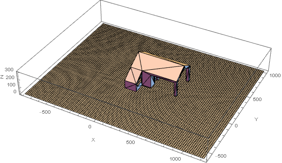
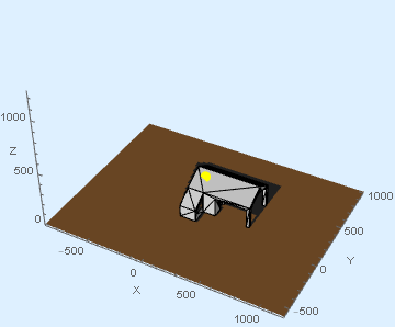
Generating The Projection Surface

The house should look like its casting it's shadow onto the earth so we define a list of points which represent the discrete plane it stands on. Each ray is a line drawn between each point on the projection surface and the position of the scene's light source.

(* rayRefinement *)
ref = 20;
(* the height of the projection surface *)
planeZoffset = 0;
(* the discrete projection surface - each point is the origin of a \
ray *)
projectionPts = 
  Catenate[Table[{x, y, planeZoffset}, {x, -900, 1200, ref}, {y, -600,
      1000, ref}]];

Graphics3D[{
  Polygon[polyPoints],
  Cuboid /@ ({##, ## + {ref, ref, 0}} & /@ projectionPts)
  }, Axes -> True, AxesLabel -> {"X", "Y", "Z"}, ImageSize -> Large]

Specifying A Light Source

The light source is typically a continuous BSplineFunction which is sampled according to the number of frames the user wants. But it may also be a discrete list of 3D points too (in which case the number of frames is equal to the length of the list).

Using a modification of a SunPosition example in the documentation, a list of the 3D Cartesian positions of the sun between sunrise and sunset, with a time step 30 minutes, is produced.

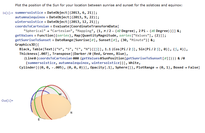
solarPositionPts0[location_:Here, date_:DateValue[Now,{"Year","Month","Day"}],tSpec_:{30,"Minute"}]:=
Evaluate[CoordinateTransformData["Spherical"->"Cartesian","Mapping",{1,\[Pi]/2-(#2 Degree),2Pi-(#1 Degree)}]]&@@@(Function[{series},Map[QuantityMagnitude,series["Values"],{2}]]@SunPosition[location,DateRange[Sunrise[#],Sunset[#],tSpec]&[DateObject[date]]])

solarPositionPts[Here, DateObject[{2017, 6, 1}], {30, "Minute"}]

{{0.4700, -0.88253, -0.0155}, {0.4026, -0.91178, 0.0809},...,{0.4219, 0.90493, 0.0554}}

It's easier to rotate the sun's path rather than the model and projection plane. Different transforms may also be applied to best-fit the path into the scene.

solarXoffset = 0;
solarYoffset = 0;
solarZoffset = 0;
zRotation = \[Pi]/3.5;
scale = 1300;

sourceSpec = 
  RotationTransform[zRotation, {0, 0, 1}][
    # + {solarXoffset, solarYoffset, solarZoffset} & /@ (solarPositionPts[Here, DateObject[{2017, 6, 1}], {30, "Minute"}] scale)
  ];

lightingPath = BSplineCurve[sourceSpec];

Specify A Frame Count

A frame count must be specified to discretize the light path into 3D points. Each of these points forms the end of each ray. If the light source is a discrete list, then its length is used to infer the frame count instead and does not need specifying by the user.

frameCount = 30;

Constructing The Scene

Now we can preview the scene

Graphics3D[{
  Polygon[polyPoints],
  Cuboid /@ ({##, ## + {ref, ref, 0}} & /@ projectionPts),
  lightingPath,
  {Darker@Yellow, PointSize[0.03], 
   Point[BSplineFunction[sourceSpec] /@ Range[0, 1, N[1/frameCount]]]}
  }, Axes -> True, AxesLabel -> {"X", "Y", "Z"}, ImageSize -> Large]

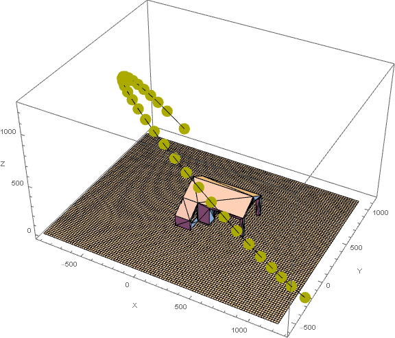
All paramaters have been set, it's time to construct the scene. Specifying a continuous lighting path must be done using a BSPlineCurve.

scene = newScene[bvh2, lightingPath, frameCount, ref, projectionPts]

Processing A Scene For Shadow Mapping

The BVH optimises the ray caster by reducing the number of polygons to search against for an intersection. If the ray intersects with the BVH root box then a breadth-first search along the BVH tree is initiated. Starting with the root box,the out-components are selected by their intersection with a ray and are used as roots for the search's next level.

(* select peripheral out-components of root box that intersect with ray *)
intersectingSubBoxes[BVHObj_,initialVertex_,rayOrigin_,raySource_]:=Select[Rest[VertexOutComponent[BVHObj["Tree"],{initialVertex},1]],intersectRayBox[#,rayOrigin,raySource]==True&];

(* for root box intersecting rays, find which leaf box(es) intersect with ray *)
BVHLeafBoxIntersection[BVHObj_,rayInt_,rayDest_]:=Block[{v0},
(*initialize search *)v0=intersectingSubBoxes[BVHObj,VertexList[BVHObj["Tree"]][[1]],rayInt,rayDest];
(* breadth search *)
If[v0=={},Return[v0],
While[
(* check that vertex isn't a polygon - true if !0.  Check that intersection isn't empty *)
AllTrue[VertexOutDegree[BVHObj["Tree"],#]&/@v0,#=!=0&],
v0=Flatten[intersectingSubBoxes[BVHObj,#,rayInt,rayDest]&/@v0,1];
If[v0==={},Break[]]
];
Return[v0];
]
];

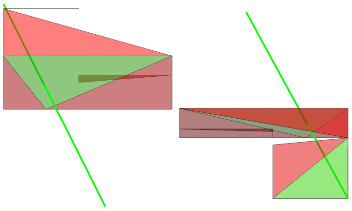
The code below generates a visualisation of this process using the input data from the scene generated.

raySource = scene["ProjectionPoints"][[3700]];
rayDestination = scene["FrameData"][16]["SourcePosition"];

lv1Intersection = 
  BVHLeafBoxIntersection[bvh, raySource, rayDestination];
lv2Intersection = 
  BVHLeafBoxIntersection[bvh2, raySource, rayDestination];

lv1Subgraph = 
  Subgraph[Graph[EdgeList[bvh2["Tree"]]], 
   First[VertexList[bvh2["Tree"]]] \[DirectedEdge] # & /@ 
    lv1Intersection];
lv2Subgraphs = Subgraph[Graph[EdgeList[bvh2["Tree"]]], Flatten[Table[
     lv1Intersection[[
         i]] \[DirectedEdge] # & /@ (Intersection[#, 
           lv2Intersection] & /@ ((Rest@
              VertexOutComponent[bvh2["Tree"], #] & /@ 
            lv1Intersection)))[[i]],
     {i, 1, Length[lv1Intersection], 1}
     ], 1]];
lbl = ((#[[1]] -> #[[2]]) & /@ (Transpose[{lv2Intersection, 
       ToString /@ Range[Length[lv2Intersection]]}]));
edgeStyle = Join[
   ReleaseHold@
    Thread[(# -> HoldForm@{Thick, Blue}) &[EdgeList[lv2Subgraphs]]],
   ReleaseHold@
    Thread[(# -> HoldForm@{Thick, Red}) &[EdgeList[lv1Subgraph]]]
   ];

rayBVHTraversal = Graph[EdgeList[bvh2["Tree"]], EdgeStyle -> edgeStyle,
   VertexLabels -> lbl,
   GraphHighlight -> lv2Intersection,
   ImageSize -> Medium];

rayModelIntersection = Graphics3D[{
    {Green, Thickness[0.01], 
     Line[{raySource, rayDestination - {220, -400, 400}}]},
    {Hue[0, 0, 0, 0], EdgeForm[{Thick, Red}], 
     Cuboid /@ lv1Intersection},
    {Hue[.6, 1, 1, .3], EdgeForm[{Thick, Blue}], 
     Cuboid /@ lv2Intersection},
    {Opacity[0.5], Polygon[polyPoints]},
    Inset @@@ 
     Transpose[{ToString /@ Range[Length[lv2Intersection]], 
       RegionCentroid /@ Cuboid @@@ lv2Intersection}]
    }];

Column[{
  Row[
   Show[rayModelIntersection, ViewPoint -> #, Boxed -> False, 
      ImageSize -> Medium] & /@ {{-\[Infinity], 0, 
      0}, {0, -\[Infinity], 0}}
   ],
  rayBVHTraversal
  }]

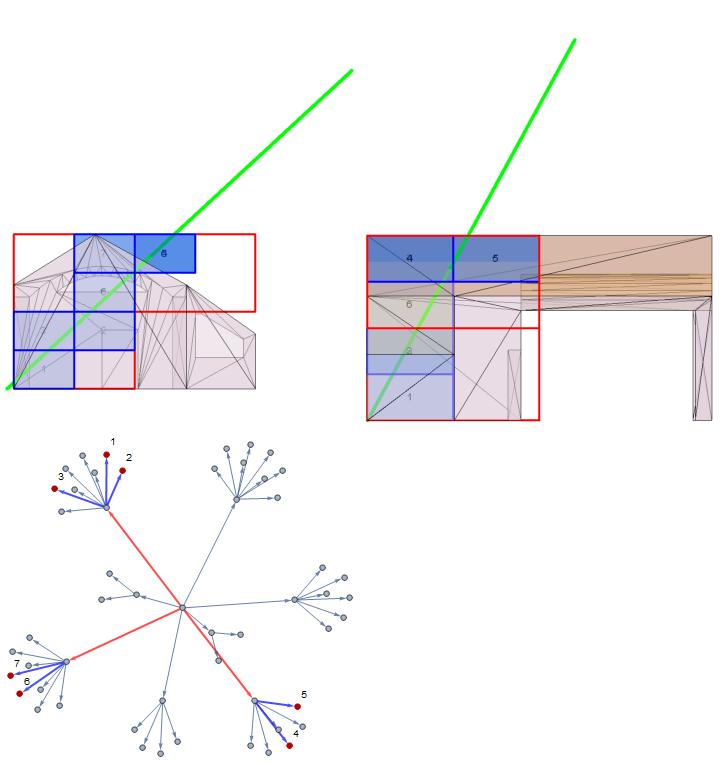
At the centre of the graph lies the vertex representing the root BV where all searches originate from. The search continues out form all vertices which have intersected with the ray.

(* test intersection between ray and object polygon via BVH search *)
intersectionRayBVH[BVHObj_,rayOrigin_,rayDest_]:=With[{
intersectionLeafBoxes=BVHLeafBoxIntersection[BVHObj,rayOrigin,rayDest]
},
Block[{i},If[intersectionLeafBoxes=!={},
Return[Catch[For[i=1,i<Length[#],i++,
Function[{thowQ},If[thowQ,Throw[thowQ]]][intersectRayTriangle[#[[1]],#[[2]],#[[3]],rayOrigin,rayDest]&@#[[i]]]
]&[DeleteDuplicates[Flatten[Lookup[BVHObj["LeafObjects"],intersectionLeafBoxes],1]]]]===True],
Return[False]
]]
];

Once the tree has been fully searched, the remaining boxes are used to lookup their associated polygons. Since the same polygon may intersect more than one box, any duplicates are deleted. A line-triangle intersection test is iteratively applied over the resultant list, breaking at the first instance of a True return. This ray has now been found to intersect a part of the 3D model thus its origin point (from the projectionPts list) will represent a single point of shadow on the projection surface. This point is stored in a list which will be used to draw the shadow for a single frame.

candidatePolys = DeleteDuplicates[Flatten[Lookup[
     bvh2["LeafObjects"],
     BVHLeafBoxIntersection[bvh2, raySource, rayDestination]
     ], 1]];

intersectingPolys = 
  Select[candidatePolys,PrimitiveIntersectionQ3D[Line[{raySource, rayDestination}],Triangle[#]] &];

rayModelIntersectionPolys = Graphics3D[{
    {Green, Thickness[0.01], 
     Line[{raySource, rayDestination - {220, -400, 400}}]},
    {Hue[1, 1, 1, .5], EdgeForm[Black], Polygon[candidatePolys]},
    {Hue[0.3, 1, 1, .5], Polygon[intersectingPolys]}
    }, Boxed -> False];

Row[Show[rayModelIntersectionPolys, ViewPoint -> #, ImageSize -> Medium] & /@ {{0, 0, \[Infinity]}, {0, \[Infinity], 0}}]

Highlighted in green, the ray has been found to intersect with 2 polygons.

The BVH search is performed for each ray, for each frame.

A scene is the input for the ray caster. If a scene is to be re-processed with different parameters then a new scene must be made. The output of the ray caster is held within a scene object. The data for each frame is associated to its frame index and is all held in the scene's "FrameData" field.

Begin processing. A status bar will indicate progress in terms of frames rendered.

scene = renderScene[scene];

it's best to save any progress by exporting afterwards.

Export["House_scene.txt", Compress[scene]]

Reviewing Processed Scenes

Each frame holds the shadow and ground data separately and have been expressed as zero-thickness cuboids (tiles) and each with side length equal to the rayRefinement parameter (recall that smaller values yield finer results).

Individual frames are accessed by their frame index. This examines frame 10.

Keys[scene["FrameData"][10]]

{"ShadowPts", "SourcePosition", "GroundPts"}

Accessing the processed scene's "FrameData" field allows a single specified frame to be drawn in Graphics3D.

Graphics3D[{
  Polygon[scene["BVH"]["PolygonObjects"]],
  {GrayLevel[0.3], EdgeForm[], 
   Cuboid /@ scene["FrameData"][10]["ShadowPts"]},
  {EdgeForm[], Cuboid /@ scene["FrameData"][10]["GroundPts"]},
  {Darker@Yellow, PointSize[0.04], 
   Point[scene["FrameData"][10]["SourcePosition"]]}
  }, Boxed -> False, Background -> LightBlue]

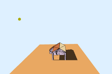
viewSceneFrame does the task above for any processed scene and specified frame. It inherits Graphics3D options as well as custom ones affecting the scene elements (shadow and ground style, toggle source drawing and gridlines).

viewSceneFrame[scene, 10, DrawGrid -> False, ShadowColor -> GrayLevel[0.3], SurfaceColor -> Lighter@Orange,  DrawSource -> True, Boxed -> False, Background -> LightBlue]

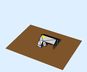
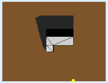
Show[viewSceneFrame[scene, 10, DrawGrid -> False, 
  ShadowColor -> GrayLevel[0.3], SurfaceColor -> Lighter@Orange, 
  DrawSource -> True, Boxed -> False, Background -> LightBlue], 
 ViewPoint -> {0, 0, \[Infinity]}]

sceneBounds = Join[
   Most[MinMax /@ Transpose[scene["ProjectionPoints"]]],
   {MinMax[
     Last /@ Values[scene["FrameData"][[All, "SourcePosition"]]]]}
   ];
viewSceneFrame[scene, 10, DrawGrid -> False, 
 ShadowColor -> GrayLevel[0.3], SurfaceColor -> Lighter@Orange, 
 DrawSource -> True, Boxed -> False, Background -> LightBlue, 
 Axes -> True, AxesLabel -> {"X", "Y", "Z"}, PlotRange -> sceneBounds]

Retaining the same options, the scene may also be animated. To ensure a smooth playback, each frame is exported as .gif into $TemporaryDirectory, imported back as a list and animated. The animation is also exported for future use.

animateScene[scene,
 DrawGrid -> False,
 ShadowColor -> GrayLevel[0.3],
 SurfaceColor -> Lighter@Orange,
 DrawSource -> True,
 Boxed -> False,
 Background -> LightBlue,
 PlotRange -> sceneBounds,
 ImageSize -> {{800}, {600}}
 ]

We can also plot the cumulative solar exposure.

All points from the projection plane which don't intersect with the model (i.e, aren't shadow points) are extracted from the scene's frames

exposure = Values[scene["FrameData"][[All, "GroundPts"]]]

The occurrences of each exposure point is tallied

tally = Tally[Flatten[exposure, 1]]

And the range of frequencies from which is generated

tallyRange = 
 Range @@ Insert[MinMax[Last /@ SortBy[tally, Last]], 1, -1]

{1, 2, 3, 4, 5, 6, 7, 8, 9, 10, 11, 12, 13, 14, 15, 16, 17, 18, 19, \
20, 21, 22, 23, 24, 25, 26, 27, 28, 29, 30}

A color scale corresponding to the range of frequencies from above will be used to colorize the plot

colorScale = 
 ColorData["SolarColors", "ColorFunction"] /@ Rescale[tallyRange]

Replacement rules are used to replace each exposure point's frequency with it's corresponding color

colorScaleRules = Thread @@ {tallyRange -> colorScale}

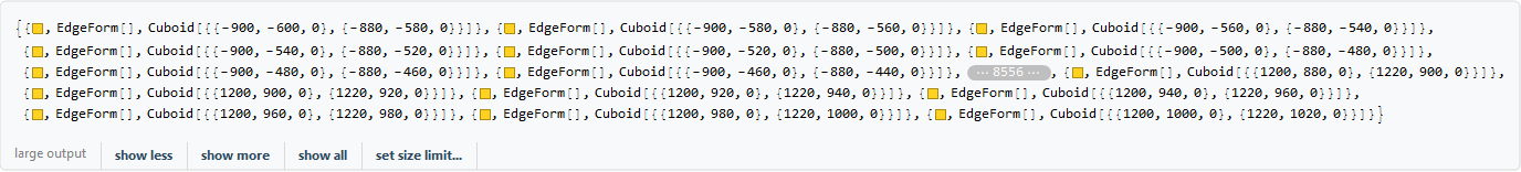
The resultant exposure map is a list of tiles, each coloured according to it's positional frequency.

heatMap = 
 Insert[MapAt[Cuboid, 
     Reverse@MapAt[Replace[colorScaleRules], #, -1], -1], EdgeForm[], 
    2] & /@ tally

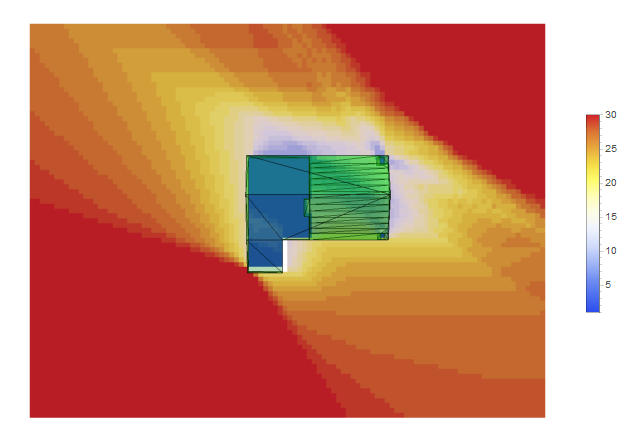
Finally, the map is drawn. It's still a Graphics3D object so it may be rotated and viewed from any angle.

Row[{
  Show[Graphics3D[{
     {Opacity[0.3], Green, Polygon[scene["BVH"]["PolygonObjects"]]},
     heatMap
     }, Boxed -> False, ImageSize -> Large], ViewPoint -> Above],
  BarLegend[{"SolarColors", MinMax[tallyRange]}]
  }]

The process of generating an exposure map forms a function within the GeometricIntersections3D package.
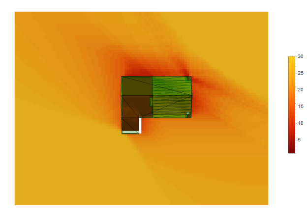
Alternative color schemes may also be specified.

sceneExposureMap[scene, "TemperatureMap"]

The bar scale for the exposure plot measures duration in frames but a time scale may be recovered. Given that the solar path used to light the scene lasts about 14 hours and the scene was rendered for 30 frames, that gives about 30 minutes per frame.

dailySunHours = 
 UnitConvert[DateDifference[Sunrise[], Sunset[]], 
  MixedRadix["Hours", "Minutes", "Seconds"]]

dailySunHours/30

This has been a very rewarding project with some exciting potentials beyond computer graphics. Indeed, much optimisations can be made to the intersections package.
The different methods of space partitioning for BVH construction should be investigated as the one currently employed is rather rudimentary. Anti-aliasing methods to be investigated also.

Both the House and Sundial processes are documented in the notebooks attached. All necessary data may also be downloaded to save time.

Attachments: