Students in introductory statistics courses learn to describe data, distributions, regression, probability, statistical inference, confidence intervals, and hypothesis tests with applications in the real world. Occasionally, hand-calculation and table-reading hinder students from engaging in the purposeful use of mathematics. In my Wolfram Summer School 2017 project, lecture notes are created using Wolfram Language so that students can visualize and enjoy statistics by becoming immersed in the context.

The goal is to create a statistics course that provides opportunities for students to experience the following elements of computational thinking: finding patterns, exploring algorithms, developing algorithms, and applying computational thinking.

Finding Patterns

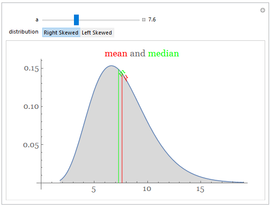
In the first module of the course, students learn how to describe data. For example, the center of a distribution is a typical value that represents the group. When we try to find the patterns for how the shape of the distribution influences the mean and median, we need to examine many histograms. In a traditional statistic class, students produce a histogram by (1) sort the data, (2) determine the number of classes, (3) calculate the class width, (4) choose the first lower class limit, (5) list all the class limits, (6) make a frequency table, then (7) draw the histogram. It usually takes minutes for the students to practice this procedure, even though they are working on some tragically small data set. To introduce meaningful real-world data, it will be necessary to use a programming language, and it is a great way to see what is possible.

Step 1: load the real-world data.

ResourceData["Sample Data: University Salaries"]
data = GroupBy[ResourceData["Sample Data: University Salaries"], "Department"][All, All, "Salary"]

Step 2: generate a histogram and plot the mean and median of the data.

d = 2;
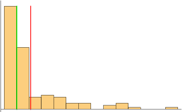
hist = Histogram[data[[d]], Ticks -> None]
mean = QuantityMagnitude[Mean[data[[d]]]]
median = QuantityMagnitude[Median[data[[d]]]]
Show[hist, 
 ContourPlot[{x == mean}, {x, mean - 1, mean + 1}, {y, 0, 50}, 
  ContourStyle -> Red, ColorFunction -> Automatic, Frame -> False, 
  Axes -> True], 
 ContourPlot[{x == median}, {x, median - 1, median + 1}, {y, 0, 50}, 
  ContourStyle -> Green, ColorFunction -> Automatic, Frame -> False, 
  Axes -> True]]

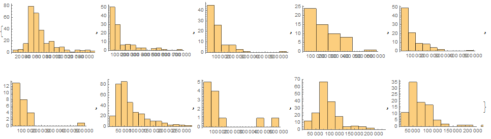
Step 3: generate a list of histograms and find the pattern.

Table[Histogram[data[[i]]], {i, 10}]

Step 4: create activities that involve manipulating existing code with no prior experience in programming required.

Exploring Algorithms

Here is another example of integrating computational thinking into the classroom content, where students see what is possible using algorithms. In previous lessons, students learned that probability distributions for discrete random variables can be visualized with histograms. Each value of a discrete variable has a probability, and this probability is the area of a corresponding bar on a probability histogram. Below is a histogram of 5000 randomly selected men's heights.

data = RandomVariate[NormalDistribution[69, 2.5], 5000];
Histogram[data,Automatic,"Probability"]

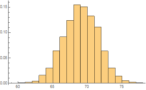
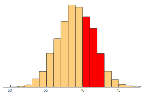
Students can estimate the probability of a man being between 71 and 73 inches tall by finding the area of the corresponding bar.

cedF[{{xmin_, xmax_}, {ymin_, ymax_}}, ___] := {If[71 <= xmax <= 73, 
    RGBColor[1, 0, 0], Sequence[]], 
   Rectangle[{xmin, ymin}, {xmax, ymax}, RoundingRadius -> 1]};
Histogram[data, ChartElementFunction -> cedF, Axes -> {True, False}]

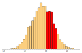
To allow more flexibility in the types of probabilities we can estimate (such as between 70.5 and 72.5 inches), it makes sense to use thinner bars.

cedF[{{xmin_, xmax_}, {ymin_, ymax_}}, ___] := {If[
    70.5 <= xmax <= 72.5, RGBColor[1, 0, 0], Sequence[]], 
   Rectangle[{xmin, ymin}, {xmax, ymax}, RoundingRadius -> 1]};
Histogram[data, {0.5}, ChartElementFunction -> cedF, 
 Axes -> {True, False}]

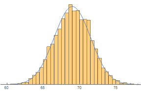
Note that the outline of the histogram can be approximated nicely by a smooth curve.

Show[Histogram[data, {0.5}, "PDF"], 
 Plot[PDF[NormalDistribution[69, 2.5], x], {x, 60, 80}], 
 Axes -> {True, False}]

With extremely thin bars, it makes sense to use a smooth curve to model the heights of the bars. Areas under such curves represent probabilities. The total area under a probability curve is 1.

Show[Histogram[
  RandomVariate[NormalDistribution[69, 2.5], 100000], {0.1}, "PDF"], 
 Plot[PDF[NormalDistribution[69, 2.5], x], {x, 60, 80}], 
 Axes -> {True, False}]

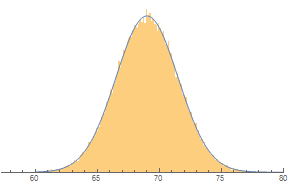
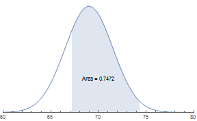
With a continuous curve, we can use mathematical formulas to find any area under the curve. The area represents probability. The distribution of probabilities under the curve forms a continuous probability distribution.

dist = PDF[NormalDistribution[69, 2.5], #] &;
p1 = Plot[dist@x, {x, 60, 67.2}, Filling -> None, 
   PlotRange -> {{60, 80}, All}, Axes -> {True, False}];
p2 = Plot[dist@x, {x, 67.2, 74.3}, Filling -> Axis, 
   PlotRange -> {{60, 80}, {0, 1}}, Axes -> {True, False}];
p3 = Plot[dist@x, {x, 74.3, 80}, Filling -> None, 
   PlotRange -> {{60, 80}, All}, Axes -> {True, False}];
Show[p1, p2, p3, Epilog -> { Text["Area = 0.7472", {70, 0.05}]}]

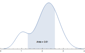
Using Wolfram Language, we can calculate the probability of any distribution.

\[ScriptCapitalD] = 
  MixtureDistribution[{1, 5}, {NormalDistribution[1, .3], 
    NormalDistribution[2.3, .5]}];
dist2 = PDF[\[ScriptCapitalD], #] &;
p1 = Plot[dist2@x, {x, 0, 1.3}, Filling -> None, 
   PlotRange -> {{0, 4}, All}, Axes -> {True, False}];
p2 = Plot[dist2@x, {x, 1.3, 2.6}, Filling -> Axis, 
   PlotRange -> {{0, 4}, {0, 1}}, Axes -> {True, False}];
p3 = Plot[dist2@x, {x, 2.6, 4}, Filling -> None, 
   PlotRange -> {{0, 4}, All}, Axes -> {True, False}];
Show[p1, p2, p3, Epilog -> { Text["Area = 0.61", {2, 0.1}]}]
NumberForm[
  Probability[1.3 <= x <= 2.6, x \[Distributed] \[ScriptCapitalD]], 
  4];

In conclusion, integrating computational thinking in the classroom provides students with opportunities to explore meaningful topics. The notebooks that I created can be found on GitHub: https://github.com/JieFrye/WSS17