Abstract
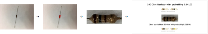
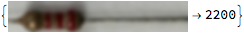
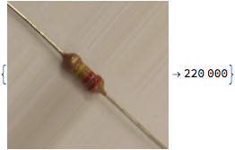
Goal of the project: To output the value of a resistor given a photo of it. The photos are intended to be taken in a white background, like from a white paper sheet and with a cellphone camera.
Summary of work: Many samples are used in a Classifier, leaving as result a logistic regression, all training and test samples were rotated and cropped automatically. The resistor position is found using morphological components, then the picture is cropped and rotated leaving the resistor to cover the majority of the picture, using the Classifier we obtain the final result.
Results and future work: The project is limited to a small set of resistors to which it can calculate the value. The next step is to either to crop the color bands of the resistor, and use machine learning in a similar way to determine the color of each of the bands of the resistor, or improve the current machine learning methods to raise the extent of the project.
First approach
For the first attempt to solve this problem the method suggested in the Lecture Notes in Computer Science where a similar problem is being solved. The difference was that the resistor photos were taken in an environment where the light is controlled, reducing the glare and shadows.
The first step was to obtain the background color of the image, this was originally done calculating the mean of the pixels near the edges of the picture, in this case it was done obtaining a mask to identify the background and calculating the mean of all the pixels in it.
img = 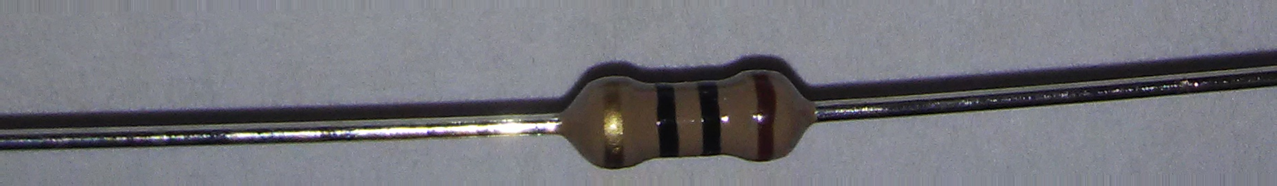
   img = ImageAdjust[ImageResize[img, {500}]];
   img = ColorConvert[RemoveAlphaChannel[img],"RGB"];
    meanColorMask[image_,mask_ ]:= Module[
    {toRemove,imgList},
    toRemove = PixelValuePositions[mask, Black];
    imgList = Transpose @ ImageData[image];
    imgList = Delete[imgList, toRemove];
    RGBColor[Mean[Catenate @ imgList]]
    ]
getBackColor[image_] := meanColorMask[image, ColorNegate @ AlphaChannel[RemoveBackground[image]]];
backColor = getBackColor[img]

This color is extracted from the image, then the result of that is converted to grayscale.
absoluteSubstract[image_, color_] := ImageApply[
	MapThread[
		Abs[#1 - #2]&,
		{Flatten[#],Flatten[List @@ color]}
	]&,
	image
]
substracted = absoluteSubstract[img, backColor]
monochromatic = ColorConvert[substracted,"Grayscale"]
From here we calculate a threshold we are going to use to separate the resistor from the background. A threshold that maximizes the variance between the rows and columns lower and higher than the threshold. Then crop the image based on the values that were higher than it. This method is further explained in [1] and [2].
 threshold[n_] := Module[
	{num, p, \[Omega], \[Mu], \[Mu]T, maxK, max\[Sigma], \[Sigma]2B, temp, k},
	num = Total[n];
	p = n / num;
	\[Omega] := Sum[p[i],{i,0,#}]&;
	\[Mu] := Sum[(i+1) * p[i], {i, 0, #}]&;
	\[Mu]T = \[Mu][255];
	\[Sigma]2B[x_Integer] := Module[
		{\[Mu]k, \[Omega]k},
		\[Omega]k = \[Omega][x];
		\[Mu]k = \[Mu][x];
		If[ \[Omega]k != 0 && \[Omega]k != 1,
			((\[Mu]T*\[Omega]k - \[Mu]k)^2) / (\[Omega]k * (1 - \[Omega]k)),
			-1
		]
	];
	max\[Sigma] = 0;
	maxK = 255;
	For[k = 0, k < 255, k++,
		temp = \[Sigma]2B[k];
		If[ NumberQ[temp] && temp > max\[Sigma],
			max\[Sigma] = temp;
			maxK = k;
		]
	];
	maxK
]
matr = ImageData[monochromatic];
verMean = Map[
	Mean[Flatten[#]]&,
	matr
];
verMean = Round[verMean * 255];
horMean = Map[
	Mean[Flatten[#]]&,
	Transpose[matr]
];
horMean = Round[horMean * 255];

horFrequency = Counts[Catenate[{horMean,Range[0,255]}]] - 1;
verFrequency = Counts[Catenate[{verMean,Range[0,255]}]] - 1;
verThreshold = threshold[verFrequency];
horThreshold = threshold[horFrequency];

verPlot = DiscretePlot[
	verMean[[x]],
	{x, 1, Length[verMean]},
	PlotRange->All,
	ImageSize->Medium
];
verThresholdPlot = Plot[
	verThreshold,
	{x, 1, Length[verMean]},
	PlotRange->All,
	ImageSize->Medium,
	PlotStyle->{Red}
];

horPlot = DiscretePlot[
	horMean[[x]],
	{x, 1, Length[horMean]},
	PlotRange->All,
	ImageSize->Medium
];
horThresholdPlot = Plot[
	horThreshold,
	{x, 1, Length[horMean]},
	PlotRange->All,
	ImageSize->Medium,
	PlotStyle->{Red}
];

xPos = Values @ Cases[
	MapIndexed[#1->First[#2]&, horMean],
	(x_->y_)/;x>= horThreshold
];
xStart = Min[xPos];
xEnd = Max[xPos];

yPos = Values @ Cases[
	MapIndexed[#1->First[#2]&, verMean],
	(x_->y_)/;x>= verThreshold
];
yStart = Min[yPos];
yEnd = Max[yPos];

segmented = ImageTake[
	img,
	{yStart, yEnd},{xStart, xEnd}
];
xStartLine = Graphics @ Line[{{xStart, 0},{xStart, 255}}];
xEndLine = Graphics @ Line[{{xEnd, 0},{xEnd, 255}}];
yStartLine = Graphics @ Line[{{yStart, 0},{yStart, 255}}];
yEndLine = Graphics @ Line[{{yEnd, 0},{yEnd, 255}}];
Grid[{
	{
		Show[{horPlot, horThresholdPlot, xStartLine, xEndLine}],
		Show[{verPlot, verThresholdPlot, yStartLine, yEndLine}]
	},
	{"Horizontal mean", "Vertical mean"}
}]
segmented
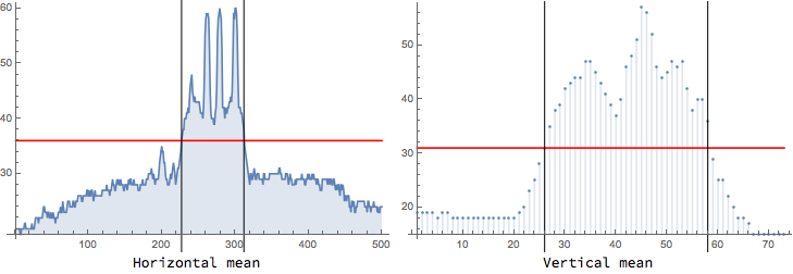

The graphs represent the average color of each of the columns and rows of the pixels of the monochromatic image. The threshold for each of them is represented with the red line and is calculated using the Otsu's method. The black lines represent the left-most, right-most columns, and top and bottom rows where the mean color is over the threshold. With those values we can cut the resistor of the image. Finally, in this approach we extract an image with a height of 15 pixels.
extracted = ImageCrop[segmented, {ImageDimensions[segmented][[1]], 15}, Center]

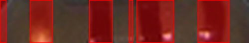
To get the color bands, the image is subtracted of the back color and made grayscale, then clustering the bars with the K-means algorithm. However, this method did not result convenient for our use case, as kept marking the glare in the resistor as part of the band.
extracted = ImageResize[extracted, {500}];
exBackColor =
ColorConvert[
	Hue @@ ImageMeasurements[ColorConvert[extracted, "HSB"], "Mean"],
	"RGB"
]
exSubs =
TotalVariationFilter @ absoluteSubstract[
	extracted,
	ColorConvert[exBackColor,"RGB"]
]
exMono = ColorConvert[exSubs, "Grayscale"]
exBinary = Binarize[exMono,Method->"Cluster"]
allX = Map[
	Interval[{Ramp[Min[#]],Ramp[Max[#]]}]&,
	Values[ComponentMeasurements[
		MorphologicalComponents[exBinary],
		"MinimalBoundingBox"
	]][[All, All, 1]]
];
allX = List @@ (IntervalUnion @@ allX);
squaresX = Polygon @ Map[
	Module[
		{min, max, height},
		min = #[[1]];
		max = #[[2]];
		height = ImageDimensions[extracted][[2]];
		{{min, 1}, {min, height}, {max, height}, {max, 1}}
	]&,
	allX
];
HighlightImage[extracted, {Red, squaresX}]


Second approach
The next approach was to use machine learning to obtain the values of the resistors. Several samples were made taking pictures from resistors on a white background, making sure they had different positions and angles. However, the training was taking too long and causing the Mathematica program to crash. Later it was concluded that the results would improve if the resistor in the photo was cropped, removing several pixels without any information the total memory needed to process the images would be lower.
For cropping the resistor from the photo, the following was made:
- Pass the photo through ImageAdjust and BrightnessEqualize rise the contrast and remove shadows from the image.
- Used the function RemoveBackground to obtain from the alpha channel a mask that would separate the resistor from the background.
- Erode said mask, so the wires in the resistor are eliminated from the mask.
- Use RegionBinarize to recover the parts of the resistor that were removed from the mask.
- Obtain the minimal bounding box and orientation angle from this resistor mask.
- Rotate and crop the image according with the previous values.
resistorCrop[image_] := Module[
	{preprocess, angle, rotated, newPoints, allX, allY, minX, minY, maxX, maxY, processed, adjusted},
	adjusted = ImageAdjust @ BrightnessEqualize[image];
	preprocess = SelectComponents[Erosion[AlphaChannel[RemoveBackground[adjusted]],10],"Count",-1];
	preprocess = RegionBinarize[adjusted,preprocess,0.15];
	processed = MorphologicalComponents[preprocess];
	angle = First @ Values[
		ComponentMeasurements[processed, "Orientation"]
	];
	rotated = ImageRotate[image, -angle, Masking->Full];
	newPoints = First @ Values[ComponentMeasurements[processed, "MinimalBoundingBox"]];
	newPoints = RotationTransform[-angle,ImageDimensions[image]/2][newPoints];
	newPoints = TranslationTransform[(ImageDimensions[rotated] - ImageDimensions[image])/2][newPoints];
	allX = newPoints[[All, 1]];
	allY = newPoints[[All, 2]];
	minX = Min[allX];
	minY = Min[allY];
	maxX = Max[allX];
	maxY = Max[allY];
	ImageTake[rotated, Ramp[ImageDimensions[rotated][[2]]-{maxY, minY}],{minX,maxX}]
]
From this function the samples would be cropped to allow the training to run faster. Some images were not cropped correctly and had to be removed.
This method can not be used for the final product though, as it takes too much time to filter the images for cropping. One way to make a faster method is to rescale the initial image smaller before obtaining the mask and at the end rescale the cropping coordinates accordingly, reducing the total pixels the program would work on. Naturally this method is less precise.
resistorLightCrop[image_] := Module[
	{preprocess, angle, rotated, newPoints, allX, allY, minX, minY, maxX, maxY, processed, adjusted, resized, prop, fullRotated},
	resized = ImageResize[image, {500}];
	prop = ImageDimensions[image][[1]] / ImageDimensions[resized][[1]];
	adjusted = ImageAdjust @ BrightnessEqualize[resized];
	preprocess = SelectComponents[Erosion[AlphaChannel[RemoveBackground[adjusted]],10 / prop],"Count",-1];
	preprocess = RegionBinarize[adjusted,preprocess,0.15];
	processed = MorphologicalComponents[preprocess];
	angle = First @ Values[
		ComponentMeasurements[processed, "Orientation"]
	];
	rotated = ImageRotate[resized, -angle, Masking->Full];
	newPoints = First @ Values[ComponentMeasurements[processed, "MinimalBoundingBox"]];
	newPoints = RotationTransform[-angle,ImageDimensions[resized]/2][newPoints];
	newPoints = TranslationTransform[(ImageDimensions[rotated] - ImageDimensions[resized])/2][newPoints];
	allX = newPoints[[All, 1]];
	allY = newPoints[[All, 2]];
	minX = Min[allX];
	minY = Min[allY];
	maxX = Max[allX];
	maxY = Max[allY];
	fullRotated = ImageRotate[image, -angle, Masking->Full];
	ImageTake[fullRotated, Ramp[ImageDimensions[fullRotated][[2]]-{maxY * prop, minY * prop}],{minX * prop,maxX * prop}]
]
SetDirectory[NotebookDirectory[]];
DumpSave["resistorLightCrop.mx", resistorLightCrop];
ResetDirectory[];
Once the images of the dataset are loaded we need to create the training set and the test set.
As the cropping method used in the training is more accurate than the one used for the final product, adding noise to the samples is needed to improve the results. This is because the method used has shown to fail sometimes in rotating the resistor in a horizontal position, especially if the wires in the resistor are bended, so more samples were the resistor is rotated to random angles were added to make the Classifier be prepared if the cropping function fails to make the rotation. Also, blurry samples using a GaussianFilter were added, to compensate loss of focus in that can be done in the photo. As for the Classifier method, a simple Classify function with a quality performance goal is used because it gave better results than forcing it to be a neural network or using a Predict function.
newBlurry[data_, n_] :=
Module[
	{toBlur},
	toBlur = RandomSample[data, n];
	toBlur/.(x_->y_):>GaussianFilter[x,15]->y
]
newRotated[data_, n_] :=
Module[
	{toRotate},
	toRotate = RandomSample[data, n];
	toRotate/.(x_->y_):>ImageRotate[x,RandomReal[{0, \[Pi]}], Masking->Full]->y
]
newBlurry[trainingSet, 1]
newRotated[trainingSet, 1]
This improved not only the accuracy for the given samples, but also the results on the final product.
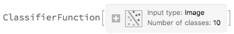
cNoParameters = Classify[trainingSet, PerformanceGoal->"Quality"]
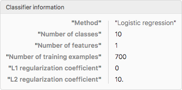
ClassifierInformation[cNoParameters]
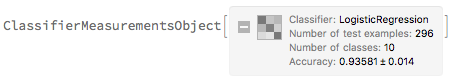
cNoParametersM = ClassifierMeasurements[cNoParameters, testSet]
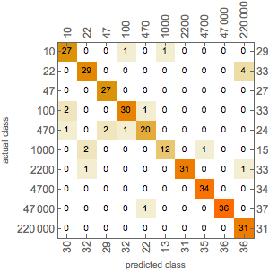
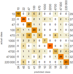
cNoParametersM["ConfusionMatrixPlot"]
Trying other methods did not give better results
cNeuralNet = Classify[trainingSet, Method->"NeuralNetwork", PerformanceGoal->"Quality", FeatureExtractor->"ImageFeatures"];
cNeuralNetM = ClassifierMeasurements[cNeuralNet, testSet]
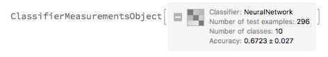
cNeuralNetM["ConfusionMatrixPlot"]
Microsite link
https://wolfr.am/mUtXyBEe
Code
https://github.com/carolinadp/WSS2017
References
[1] Mitani Y., Sugimura Y., Hamamoto Y. (2008) A Method for Reading a Resistor by Image Processing Techniques. In: Lovrek I., Howlett R.J., Jain L.C. (eds) Knowledge-Based Intelligent Information and Engineering Systems. KES 2008. Lecture Notes in Computer Science, vol 5177. Springer, Berlin, Heidelberg
[2] Otsu N. A Threshold Selection Method from Gray-Level Histograms. IEEE Transactions on Systems, Man and Cybernetics. 1979


