My goal was to create a function that could generate a 3D representation of a landscape from a topographical map. I decided to do this by building a convolution neural network that could have a grayscale topographical map as an input, and a grayscale heat map as an output. A 3D image could then be constructed from the data encoded in the heat map.

Making random maps

In order to generate enough training data for the neural network, I needed to be able to generate random artificial landscapes:

makeMountains[x_List, n_Integer] :=
 Flatten[
  Table[
   RandomVariate[
    BinormalDistribution[i, {RandomReal[], RandomReal[]}, 
     RandomReal[{-1, 1}]],
    RandomInteger[{1, 100}]
    ],
   {i, x}
   ],
  1
  ]

The function makeMountains generates a random list of n points. To turn this into a landscape, I wrote another function:

randTopo :=
 Rasterize[
  randMountain =
   SmoothHistogram3D[
    makeMountains[RandomReal[{-15, 15}, {200, 2}], 100],
    Lighting -> {White, "Ambient"},
    Mesh -> {Table[i, {i, -15 + RandomInteger[{0, 5}], 15, 6}], 
      Table[i, {i, -15 + RandomInteger[{0, 5}], 15, 6}], 30},
    PlotStyle -> White,
    MeshFunctions -> { #1 & , #2 & , #3 &},
    Boxed -> False,
    Axes -> False,
    PlotRangePadding -> None,
    ImagePadding -> None,
    ViewPoint -> {0, 0, \[Infinity]},
    PlotRange -> {{-15, 15}, {-15/1.6, 15/1.6}},
    AspectRatio -> 1/1.6
    ],
  ImageSize -> {600 1.6, 600}
  ]

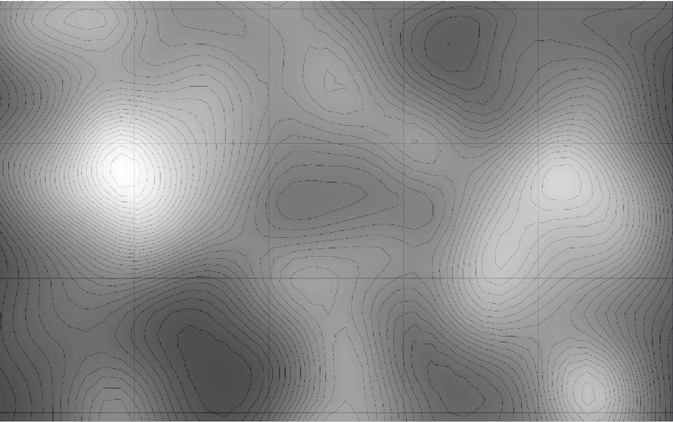
The function randMountain makes a smooth 3D histogram plot of makeMountains. The function randTopo creates an image that is a top-down view of this plot. The three types of mesh create gridlines and contour lines, which make the image look like a real topographical map. The Mesh parameter is used to make sure that the gridlines are placed slightly differently each time randTopo is used to make a map. This is done so that the neural network learns to ignore the gridlines that are present on most real maps.

I then needed to make a function that could generate a grayscale heat map that would correspond to the map generated by randTopo:

heatMap :=
 Rasterize[
  ListDensityPlot[
   pointsNew = 
    Transpose[{randMountain[[1, 1]][[All, 1]], 
      randMountain[[1, 1]][[All, 2]], 
      Rescale[randMountain[[1, 1]][[All, 3]]]}],
   Frame -> False,
   ImagePadding -> None,
   PlotRangePadding -> None,
   ColorFunction -> GrayLevel,
   AspectRatio -> 1/1.6
   ],
  ImageSize -> {600 1.6, 600}
  ]

The function heatMap accomplishes this by rasterizing a ListDensityPlot of the points from randMountain. However, the points are altered by pointsNew so that the height values are all between 0 and 1. The normalized height values are then encoded as intensity values in the grayscale ListDensityPlot. We can overlay the heat map and the random topographical map and see that the areas of higher elevation are brighter than the areas of lower elevation:

Using these randomly generated topo maps and heat maps, I created a small data set on which to train the neural network:

trainingData = Table[randTopo -> heatMap, 50];

The neural network

The next step was to build the convolution neural network. I started by defining some layers that would be used repeatedly:

Layers

convLayer1[channels_, kernelSize_, options___] :=
 NetChain[{
   ConvolutionLayer[channels, kernelSize, options],
   ElementwiseLayer[Ramp],
   BatchNormalizationLayer[]}]

convLayer2[channels_, kernelSize_, options___] :=
 NetChain[{
   ConvolutionLayer[channels, kernelSize, options],
   ElementwiseLayer[Ramp],
   BatchNormalizationLayer[],
   PoolingLayer[2, "Stride" -> 2]}]

deconvLayer1[channels_, kernelSize_, options___] :=
 NetChain[{
   DeconvolutionLayer[channels, kernelSize, options],
   ElementwiseLayer[Ramp],
   BatchNormalizationLayer[]}]

I then put these layers into a network:

mapNN = NetChain[{
   NetChain[{
     ConvolutionLayer[32, {3, 3}, "Stride" -> 2, 
      "Weights" -> Automatic],
     ElementwiseLayer[Ramp],
     BatchNormalizationLayer[]},
    "Input" -> {1, 600, 960}],
   convLayer1[64, {3, 3}, "Stride" -> 2],
   convLayer1[128, {3, 3}, "Stride" -> 2],
   convLayer2[256, {3, 3}, "Stride" -> 2],
   convLayer2[512, {3, 3}, "Stride" -> 2],
   deconvLayer1[256, {3, 3}, "Stride" -> 2],
   deconvLayer1[128, {3, 3}, "Stride" -> 2],
   deconvLayer1[64, {3, 3}, "Stride" -> 2],
   deconvLayer1[32, {3, 3}, "Stride" -> 2],
   deconvLayer1[16, {3, 3}, "Stride" -> 2],
   deconvLayer1[8, {3, 3}, "Stride" -> 2],
   deconvLayer1[1, {3, 3}, "Stride" -> 2],
   ResizeLayer[{600, 960}],
   ElementwiseLayer[LogisticSigmoid]},
  "Input" -> 
   NetEncoder[{"Image", ImageDimensions[randTopo], "Grayscale"}], 
  "Output" -> NetDecoder[{"Image", ColorSpace -> "Grayscale"}]]

The ResizeLayer is present at the end due to the loss of pixels from repeated convolution layers. It simply makes sure that the heat map output is the same size as the input image. The LogisticSigmoid keeps all of the intensity values of the heat map between 0 and 1.

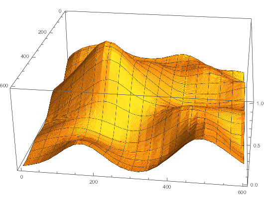
Generating the 3D landscape

The whole point of the heat map is that it has height values encoded as intensity. These values are also normalized, so in the final 3D model all of the mountains and valleys will be at the right elevation relative to each other. This way, there is no need to worry about the elevation numbers written on a real topographical map.

To make the 3D landscape, I extracted the data encoded in the heat map:

imageData = ImageData[heatMap];

mapPoints = Flatten[
   Table[{i, j, imageData[[i, j, 1]]}, {i, Length[imageData]}, {j, 
     Length[imageData]}],
   1];

I then used ListPlot3D to get the final result:

Testing

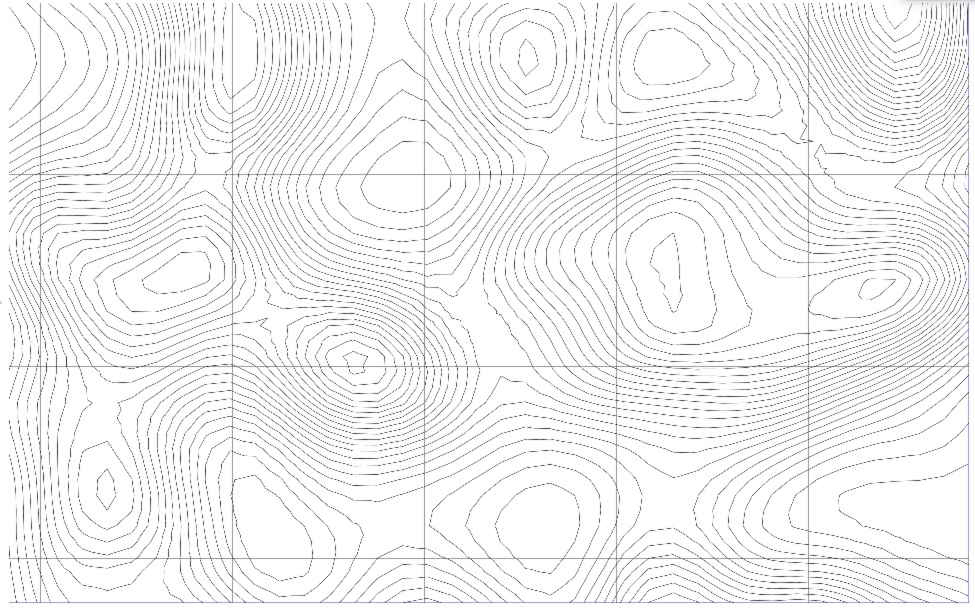
I was unable to test the neural network on a large enough data set. After being trained on 50 input/output pairs, I tried to input the following map:

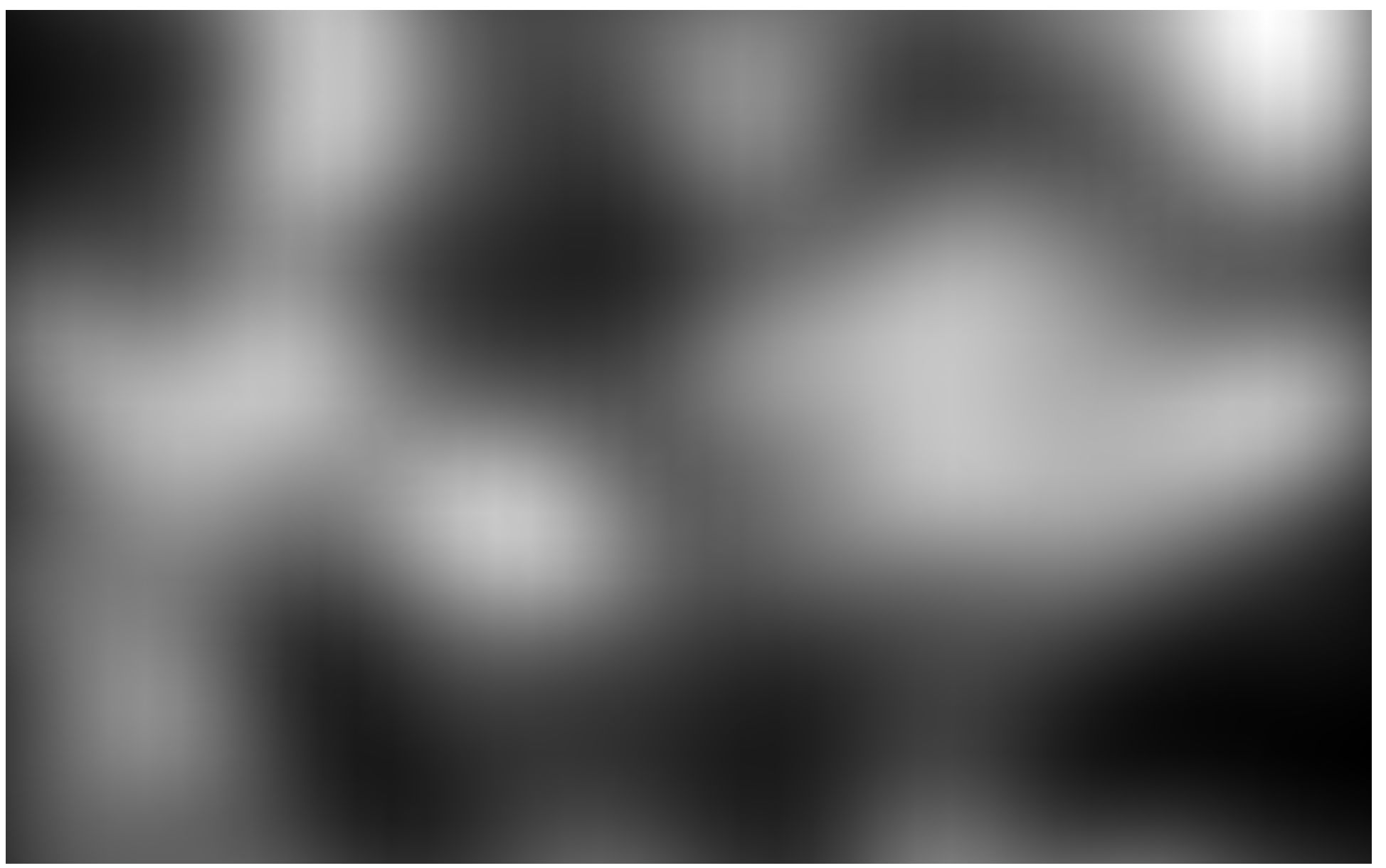
I got the following output:

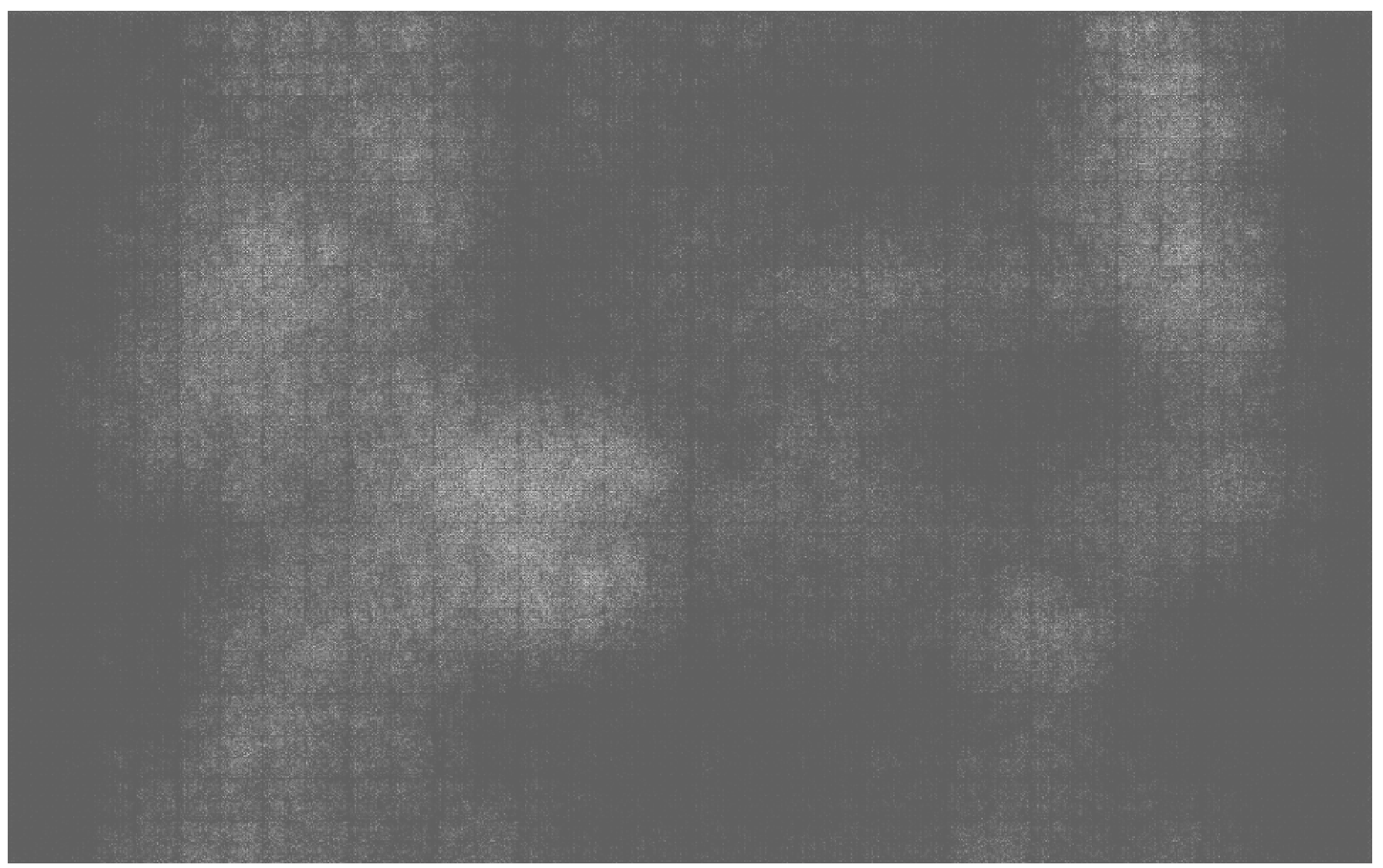
Although this heat map is far from clear or accurate, it does seem to show some of the bright spots where it is supposed to. This can be seen by comparing it to the heat map generated from the heatMap function:

Particularly on the left side of the image, the result seems pretty good for a neural network trained on such a small data set. On the right, you can see that the neural net mistook a mountain for a cone-shaped valley (there is a bright 'ring' with a dark center). With a larger set of training data, the neural network would learn that valleys are rarely steep or cone-shaped, and that contour lines that are very dense typically indicate mountains.

Notes

The results here could certainly be improved. As previously mentioned, a larger set of training data would likely produce better results. Also, there are no elevation numbers, legends, or place names on my randomly generated topographical maps. Adding these features to some of the training images might help the neural network learn to ignore them.

My full code can be found here.