Introduction

Why is the price of the electricity so high or low and varies so much between states? Does it depend on the weather? Taxes? There is actually a lot of information related to pricing electricity. In a deregulated market like in the US, the market is separated in the upstream, which generates power and supplies it to the grid and the downstream that is in charge to actually providing electricity to the users. There is a problem thought, since electricity can't be stored it has to be produced accordingly to the instant demand of the consumer market. This is where the traders come in. Being a free market, everyone can buy or sell packages of electricity that can be sold later and injected into the grid. Correct estimation of future prices is vital to traders in order to make a profit. Because there is a lot of agents in the market it is expected that the market is efficient, that is, the price should reflect all the available information. But what information is actually relevant to the price? We will explore this question from the basics.

Loading the data

In order to investigate the pricing of electricity we need first the actual prices by state and date. The U.S. Energy Information Administration (EIA) it's one of the most complete resources available, and they have a complete database of the prices (Cents per Kilowatthour). Governmental databases are not exactly pretty. This database is comprised of multiple excel files organized on directories labeled by the date they made the survey and it can be processed using the Wolfram Language.

First, since the Wolfram Language can make use of Entities to represent AdministrativeDivisions we should make a substitution rule to change every occurrence of a state name to an entity.

stateNames = {"New England","Connecticut","Maine","Massachusetts","New Hampshire","Rhode Island","Vermont","Middle Atlantic","New Jersey","New York","Pennsylvania",
              "East North Central","Illinois","Indiana","Michigan","Ohio","Wisconsin","West North Central","Iowa","Kansas","Minnesota","Missouri","Nebraska","North Dakota",
              "South Dakota","South Atlantic","Delaware","District of Columbia","Florida","Georgia","Maryland","North Carolina","South Carolina","Virginia","West Virginia",
              "East South Central","Alabama","Kentucky","Mississippi","Tennessee","West South Central","Arkansas","Louisiana","Oklahoma","Texas","Mountain","Arizona",
              "Colorado","Idaho","Montana","Nevada","New Mexico","Utah","Wyoming","Pacific Contiguous","California","Oregon","Washington","Pacific Noncontiguous","Alaska",
              "Hawaii","U.S. Total"};
stateEntitiesRule = ReplaceAll[Map[#->Interpreter["AdministrativeDivision"][#]&, stateNames], _Failure->None];

The database contains residential, commercial and industrial electricity prices. Since the industrial prices are usually less regulated we will focus our analysis on those.

residential = 2;
commercial = 4;
industrial = 6;
directories = Select[FileNames["*", NotebookDirectory[]<>"ElectricityPrices"], FileType[#] == Directory&];

electricityPricesByDate = Table[
    data = First[Import[d <> "/Table_5_06_A.xlsx"]];
    date = DateObject[data[[4, 2]]];
    statesAndPrices = Take[data, {5, -3}];
    entityStates = statesAndPrices[[All,1]] /. stateEntitiesRule;
    statePrices =  DeleteCases[Transpose[{entityStates,statesAndPrices[[All, industrial]]}], {None,_}|{__String}];
    {date,statePrices}
    ,{d,directories}
];
electricityPricesByDate = SortBy[electricityPricesByDate, First];

Now we can visualize the prices of every state.

Manipulate[
    GeoRegionValuePlot[
       electricityPricesByDate[[i,2]],
       PlotLabel->"Electricity price, " <> DateString[electricityPricesByDate[[i,1]]], 
       ImageSize->500, 
       ColorFunctionScaling->False, 
       ColorFunction->(ColorData["Rainbow"][Log[#/15+1]]&)
    ],
    {i,1,Length[electricityPricesByDate],1},
    SaveDefinitions->True
]

It looks random at plain sight. Hawaii and Alaska are overpriced compared to the rest of the country, and in the central areas there is no clear trend. Actually we should not pay much attention to Hawaii and Alaska because for the rest of the analysis we will exclude them since there is missing data relating to those states in the other databases. Also, the electricityPricesByDate list is not shaped adequately for times series analysis. We should correct that and eliminate the unnecessary states.

dates = electricityPricesByDate[[All,1]];
states = electricityPricesByDate[[1, 2, All, 1]];
prices = Transpose[electricityPricesByDate[[All, 2, All, 2]]];
electricityPricesByState = Table[{states[[i]],Transpose[{dates,prices[[i]]}]},{i, 1, Length[states]}];
electricityPricesByState = DeleteCases[electricityPricesByState, 
                                       {Entity["AdministrativeDivision",{"Alaska","UnitedStates"}],_}|{Entity["AdministrativeDivision",{"DistrictOfColumbia","UnitedStates"}],_}|
                                       {Entity["AdministrativeDivision",{"Hawaii","UnitedStates"}],_}];
electricityPricesByState = SortBy[electricityPricesByState,First];

With this we should be able to plot the price in time of every state.

plots = Map[DateListPlot[#[[All, 2]], PlotLegends -> #[[All, 1]]]&, Partition[electricityPricesByState, 5]];
Grid[Partition[plots, UpTo[3]], Frame -> All]

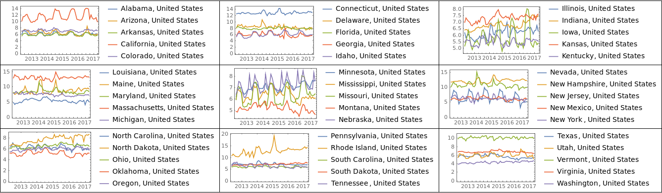
These plots are interesting because there is some noticeable periodicity and correlations between the prices. It seems worth investigating why some states seem highly correlated. For this we can start constructing a correlation matrix.

states = electricityPricesByState[[All,1]];
stateNames = Map[StringDelete[EntityValue[#,"Name"],", United States"]&,states];
prices = electricityPricesByState[[All,2,All,2]];
corrMatrix = Correlation[Transpose[prices]];

horizontalTicks = Transpose[{Range[Length[stateNames]], stateNames}];
verticalTicks = Transpose[{Range[Length[stateNames]], Map[Rotate[#,90 Degree]&, stateNames]}];
MatrixPlot[corrMatrix, FrameTicks->{{horizontalTicks, None},{verticalTicks, None}}, PlotLegends->Automatic, ImageSize->1000]

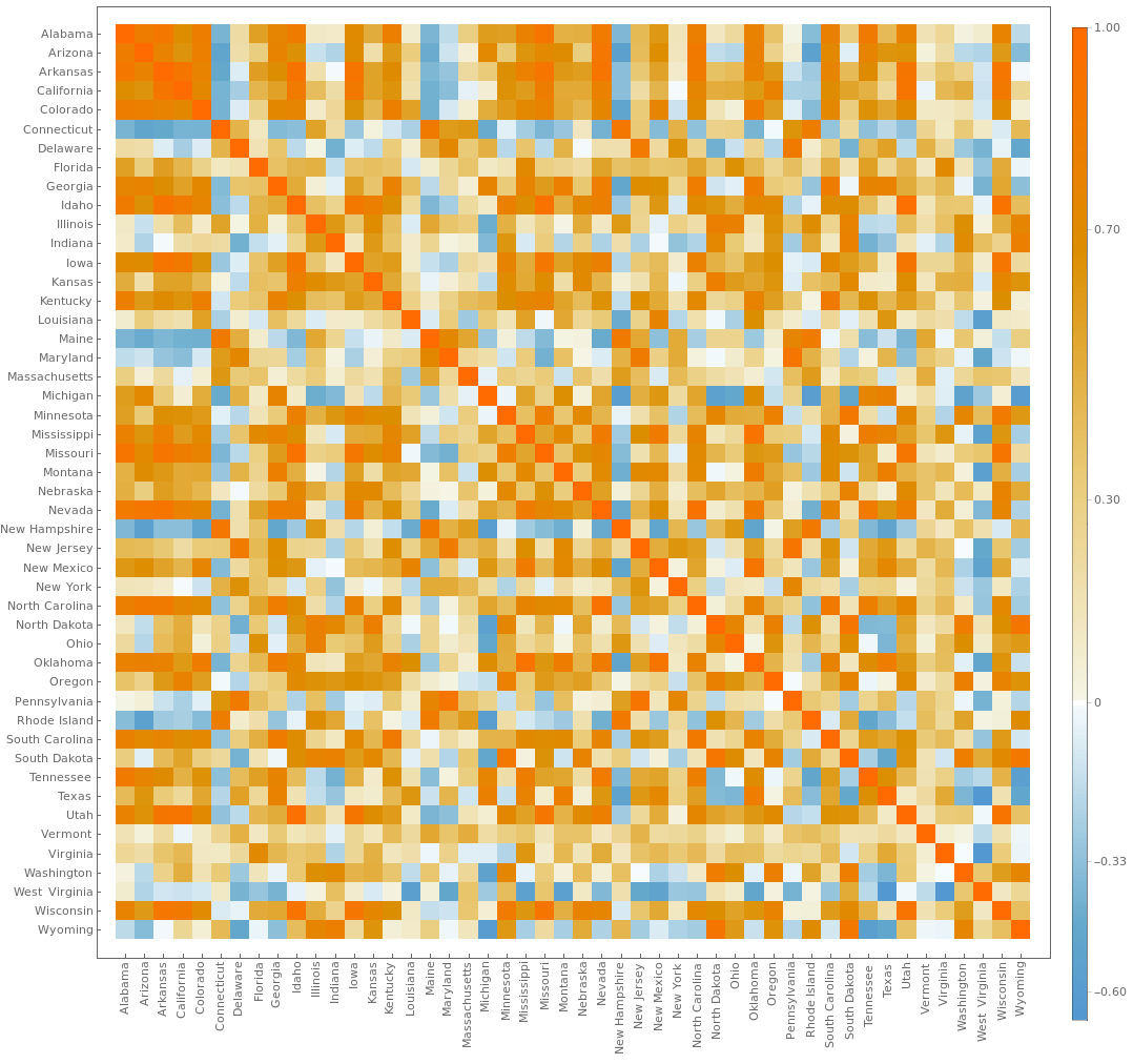
So now extracting the highly correlated states and plotting them may give us some information.

states = electricityPricesByState[[All,1]];
niceCorr = Position[corrMatrix-IdentityMatrix[Length[corrMatrix]], x_/;x>0.7];
niceCorr = DeleteDuplicates[Map[Sort, niceCorr]];
corrStates = Map[Part[states, #]&, niceCorr];
Manipulate[GeoListPlot[corrStates[[i]]],{i, 1, Length[corrStates], 1}, SaveDefinitions->True]

Now we have a lead. It seems that highly correlated states are usually geographically closer. This can be seen in more detail plotting the distribution of distances between highly correlated states.

Histogram[
    Map[QuantityMagnitude[GeoDistance[#, UnitSystem->"km"]]&, corrStates], 
    10, 
    "Probability", 
    Frame->True, 
    FrameLabel->{"Distance (km)", "Probability"}
]

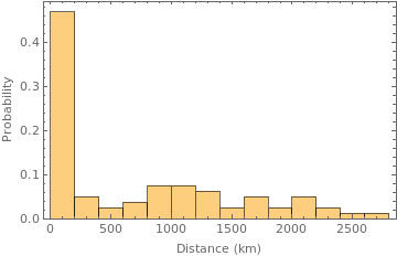
Almost 50% of the highly correlated states are geographically close. This can be due to a multitude of factors. It might be that close states usually share the same geography and climate, and that is in part true, but the actual reason lies on how the electrical grid is constructed.

The grid

Maintaining a electrical grid is a hard job, and because we use alternating current, every electrical connection of the grid must alternating at the same frequency on all the grid, and this becomes harder the larger is the region. Because of this, in the mainland of the U.S. the grid is divided into 8 regions.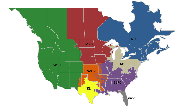

Although they can share electricity by direct current connections, each of these regions can function as an independent unit. This is the reason why many of the highly correlated states were geographically close. To visualize this using Wolfram Language we need a way to import the freely available data of the coordinates of each grid. Unfortunately Mathematica has trouble parsing some KML files, but we can just parse them manually using patterns.

data = Import[NotebookDirectory[]<>"nerc-regions.kml","XML"];
namesString = Drop[Flatten[Cases[data, XMLElement["name", {}, n_] :> n, Infinity]],1];
coordinatesString = Cases[data, XMLElement["coordinates", {}, c_] :> c, Infinity];

StringCoordToPolygon[s_String] := Module[{flattenCoord,coord},
    flattenCoord = ToExpression[StringSplit[s, Whitespace | ","]];
    coord = Partition[Drop[flattenCoord, {3, Length[flattenCoord], 3}], 2];
    Polygon[coord]
];

nercAreas = Transpose[{namesString, Map[StringCoordToPolygon[First[#]]&, coordinatesString]}];
nercAreas = DeleteCases[nercAreas, {"ASCC", _}|{"HICC", _}];

And after parsing we plot them alongside the highly correlated states. It is now clearer that many of the highly correlated states are in the same grid.

FindNercArea[state_] := Module[{nercAreasNames,nercAreasCoord,testResults,pos},
    nercAreasNames = nercAreas[[All,1]];
    nercAreasCoord = nercAreas[[All,2]];
    testResults = Map[GeoWithinQ[#, EntityValue[state, "Coordinates"]]&, nercAreasCoord];
    If[Apply[Or, testResults] == True,
       First[Extract[nercAreasNames, Position[testResults,True]]],
       None
    ]
];
nercAreaOfState = Table[{s, FindNercArea[s]}, {s, states}];

coordinates = nercAreas[[All,2]];
labels = MapThread[Text[#1, GeoPosition[Reverse[RegionCentroid[#2]]]]&, Transpose[nercAreas]];
nercAreasForPlotting = MapThread[{EdgeForm[Black], #1, #2}&, {coordinates,labels}];
Manipulate[
    Show[
       GeoGraphics[nercAreasForPlotting],
       GeoListPlot[corrStates[[i]], PlotStyle -> Directive[EdgeForm[Thick]]],
       GeoRange->"Country",
       PlotLabel->"Highly correlated states. Grid as background."
    ],
    {i, 1, Length[corrStates],1},
    SaveDefinitions->True
]

41% of the high correlated states share the same grid.

corrStatesAreas = Map[FindNercArea,corrStates, {2}];
N[Length[Select[corrStatesAreas, Apply[SameQ, #]&]]/Length[corrStatesAreas]]

0.417722

Degree days

Another factor crucial in determining the demand of electricity (and hence the price) are climate factors. One cannot however try to correlate directly the temperature to the amount of electricity consumed. This is because people don't usually turn their air conditioners or heating unless the temperature exceed some baseline interval. A better way to measure the demand caused by high and low temperatures is to use cooling and heating degree days.

Let's imagine a building where the temperature is comfortable when the outside it's at ~65 °F. If the temperature outside had a high of 90 °F and a low of 66 °F the cooling degree days are calculated as:

Mean[{90,66}]-65
13

If the high temperature was 33 °F and the low 25 ° F the heating degree days are calculated as:

65-Mean[{33,25}]
36

We can generalize this measure to a city or a state by considering the average comfortable temperature of building by zone and weighting the values by population. This tremendous amount of work is done by the National Oceanic and Atmospheric Administration of the U.S and is freely available in their ftp server. As always with governmental databases, the format is not pretty. This one consist of formatted text with each entry separated with "|", but it can be easily parsed. First we will convert the abbreviation of state names to Entities and make a rule.

stateCodes = {"AL","AR","AZ","CA","CO","CT","DE","FL","GA","IA","ID","IL","IN","KS","KY","LA","MA",
              "MD","ME","MI","MN","MO","MS","MT","NC","ND","NE","NH","NJ","NM","NV","NY","OH","OK",
              "OR","PA","RI","SC","SD","TN","TX","UT","VA","VT","WA","WI","WV","WY"};
shortStateRule = Map[# -> Interpreter["AdministrativeDivision"][#]&, stateCodes];

Then we make the parsing of the database.

FullDateToMonthly[date_] := DateObject[Map[DateValue[date,#]&,{"Year","Month"}]];
ExtractDegreeDays[txt_] := Module[{lines,dateStrings,dates,stateAndDDays,states,ddays,datesAndDDays,gatheredByMonth,datesAndDegreeDaysByMonth},
    lines = StringSplit[txt, "\n"];
    dateStrings = Drop[StringSplit[lines[[4]], "|"],1];
    dates = Map[DateObject, dateStrings];
    stateAndDDays = Map[StringSplit[#, "|"]&, Drop[lines,4]];
    states =stateAndDDays[[All,1]] /. shortStateRule;
    ddays = Map[Drop[#, 1]&, stateAndDDays];
    datesAndDDays = Map[Transpose[{dates, ToExpression[#]}]&,ddays];
    datesAndDegreeDaysByMonth = Table[
       gatheredByMonth = GatherBy[dh, DateValue[First[#],"Month"]&];
       Map[{FullDateToMonthly[#[[1,1]]], Total[#[[All, 2]]]}&, gatheredByMonth]
       ,{dh,datesAndDDays}
    ];
    Transpose[{states,datesAndDegreeDaysByMonth}]
];

directories = Select[FileNames["*",NotebookDirectory[]<>"DegreeDays"],FileType[#]==Directory&];

heatingDegreesByStateYearly = Table[ExtractDegreeDays[Import[d <> "/StatesCONUS.Heating.txt"]], {d, directories}];
heatingDegreesByState = Table[{t[[1,1]], Flatten[t[[All,2]], 1]}, {t, Transpose[heatingDegreesByStateYearly]}];

coolingDegreesByStateYearly = Table[ExtractDegreeDays[Import[d <> "/StatesCONUS.Cooling.txt"]], {d, directories}];
coolingDegreesByState = Table[{t[[1,1]], Flatten[t[[All,2]], 1]}, {t, Transpose[coolingDegreesByStateYearly]}];

Since we will be working with multiple database it is a good idea to make all the dates match.

dates = Sort[electricityPricesByDate[[All,1]]];
SelectInDateRange[data_] := Select[data, First[dates] <= First[#] <= Last[dates]&];
heatingDegreesByState = MapAt[SelectInDateRange, heatingDegreesByState, {All,2}];
coolingDegreesByState = MapAt[SelectInDateRange, coolingDegreesByState, {All,2}];
heatingDegreesByState = SortBy[heatingDegreesByState, First];
coolingDegreesByState = SortBy[coolingDegreesByState, First];

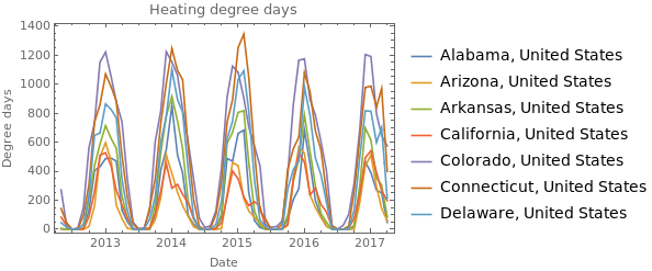
Then we can plot some of them.

pltData = Take[heatingDegreesByState, 7];
DateListPlot[pltData[[All,2]], FrameLabel->{"Date", "Degree days"}, PlotLegends -> pltData[[All,1]], PlotLabel -> "Heating degree days"]

pltData = Take[coolingDegreesByState,7];
DateListPlot[pltData[[All,2]], FrameLabel->{"Date", "Degree days"}, PlotLegends -> pltData[[All,1]], PlotLabel -> "Cooling degree days"]

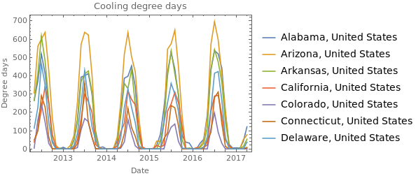
When correlating degree days with electricity prices a strange behavior becomes apparent. The price can be positively or negatively correlated with both heating and cooling degree days, and it varies a lot from state to state.

DegreeDaysCorrPlots[data_]:=Module[{states, degreeDays, prices, stateName, corrString},
    states = electricityPricesByState[[All,1]];
    RandomSample[
       Table[
         degreeDays = data[[s,2,All,2]];
         prices = electricityPricesByState[[s,2,All,2]];
         stateName = StringDelete[states[[s]]["Name"], ", United States"];
         corrString = "Correlation: "<>ToString[Correlation[degreeDays,prices]];
         ListLinePlot[{Standardize[degreeDays], Standardize[prices]}, Frame->True, FrameLabel->{"Index","Value"}, PlotLegends->{"Standardized degree days","Standardized prices"},
         PlotLabel->stateName<>"\n"<>corrString
       ]
       ,{s, 1, Length[states]}
       ],
       4
    ]
];

heatingDegreeDaysCorrPlots = DegreeDaysCorrPlots[heatingDegreesByState];
coolingDegreeDaysCorrPlots = DegreeDaysCorrPlots[coolingDegreesByState];
heatingGridElements = Join[{{Style["Heating degree days", 20, Red], SpanFromLeft}}, Partition[heatingDegreeDaysCorrPlots, 2]];
coolingGridElements = Join[{{Style["Cooling degree days", 20, Blue], SpanFromLeft}}, Partition[coolingDegreeDaysCorrPlots, 2]];

Grid[heatingGridElements, Frame->All]
Grid[coolingGridElements, Frame->All]

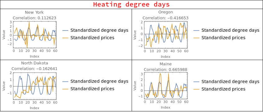
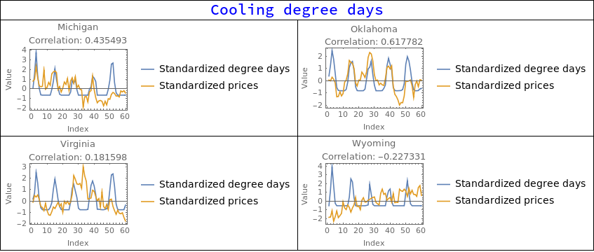
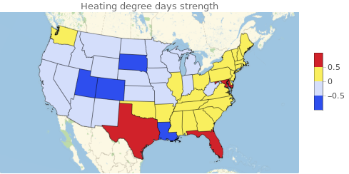
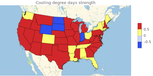
This is where things get interesting because there is no certain way to tell what is happening here. It could be that some states are more dependent on heating equipment than cooling. It could be that some states rely on solar power, explaining negative correlations with cooling degree days. It could be that certain industries rely on a specific climate to lower consumption. It could be many things, but luckily we don't actually need to know all these factors to actually predict prices. We can make the assumption that whatever the factors that make the correlations behave like they do, these factors will be constant in time (or at least change very slowly). With this in mind we can then define two values ? and ? of the "strength" of heating degree days and cooling degree days respect to price changes. Then we find the optimum values of ? and ? to maximize correlation between degree days and electricity prices. ? and ? will be very important to predict the prices since in the we are encoding a lot of information about the state.

statealphabetaparamsWCorr = Table[
    prices = electricityPricesByState[[s, 2, All, 2]];
    hd = heatingDegreesByState[[s, 2, All, 2]];
    cd = coolingDegreesByState[[s, 2, All, 2]];
    alphabetatbl = Flatten[Table[{alpha, beta, Correlation[{alpha, beta}.{hd, cd},prices]}, {alpha, -1, 1, 0.03}, {beta, -1, 1, 0.03}], 1];
    {states[[s]], First[MaximalBy[alphabetatbl, Last]]}
    ,{s, 1, Length[states]}
];

statealphabetaparams = MapAt[Drop[#, -1]&, statealphabetaparamsWCorr, {All, 2}];
GeoRegionValuePlot[Transpose[{statealphabetaparams[[All, 1]], statealphabetaparams[[All, 2]][[All, 1]]}], ColorFunction->"TemperatureMap", PlotLabel->"Heating degree days strength"]
GeoRegionValuePlot[Transpose[{statealphabetaparams[[All, 1]], statealphabetaparams[[All, 2]][[All, 2]]}], ColorFunction->"TemperatureMap", PlotLabel->"Cooling degree days strength"]

GDP and prices of fuel

One factor that is related to prices is the GDP of the state. This is because is a measure of how well the economy is doing, and this affect wages and investment in infrastructure. The GDP can be obtained as an EntityProperty, but the problem is that is delivered in a daily time series. For our purposes we will have to resample it to monthly values.

DateToYearly[date_] := DateObject[{DateValue[date,"Year"]}];

dates = Sort[electricityPricesByDate[[All,1]]];
FindStateGDPByMonth[state_,datefrom_,dateto_] := Module[{gdpTS, gdpValues, datesMissing, fillArr},
    gdpTS = EntityValue[state, EntityProperty["AdministrativeDivision","GrossDomesticProduct", {"Date"->Interval[{DateToYearly[datefrom],DateToYearly[dateto]}]}]];
    gdpValues = MapAt[DateToYearly, Normal[QuantityMagnitude[gdpTS]], {All,1}];
    gdpValues = MapAt[#/10^10&, gdpValues, {All,2}]; (* Adjust the magnitude so I don't get big numbers that crashes the predictor *)
    gdpValues = Flatten[Table[Map[If[DateWithinQ[g[[1]],#],{#,g[[2]]}, Nothing]& ,dates], {g,gdpValues}], 1];
    datesMissing = Complement[dates, gdpValues[[All,1]]]; (* Since GDP of current year can't be obtained I will shamefully use the last known value *)
    fillArr = ConstantArray[Last[gdpValues][[2]], Length[datesMissing]];
    gdpValues = Join[gdpValues, Transpose[{datesMissing, fillArr}]];
    Return[gdpValues];
];
gdps = Table[{s, FindStateGDPByMonth[s, First[dates], Last[dates]]}, {s, states}];

The we can get a nice visualization.

Manipulate[
    GeoRegionValuePlot[
       Transpose[{gdps[[All,1]], gdps[[All,2,t]][[All,2]]}],
       PlotLabel -> "GDP, " <> DateString[dates[[t]]],
       ColorFunctionScaling -> False,
       ColorFunction->(ColorData["Rainbow"][Log[#/100+1]]&)
    ],
    {t,1,Length[dates], 1},
    SaveDefinitions->True
]

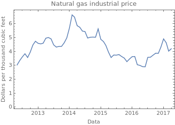
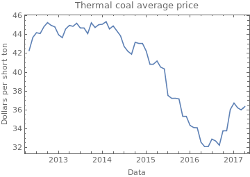
Lastly it is expected that electricity prices will be dependent on the actual commodities needed to generate it, like thermal coil and natural gas (I didn't consider uranium because of it's long lifespan). Having their prices in time will greatly help the predictor. The data was obtained from the EIA and from Quandl.

naturalGasIndustrialPriceAll = Import[NotebookDirectory[]<>"CommodityPrices/United_States_Natural_Gas_Industrial_Price.csv"];
naturalGasIndustrialPriceAll = SortBy[MapAt[DateObject, naturalGasIndustrialPriceAll,{All,1}], First];
dates = Sort[electricityPricesByDate[[All,1]]];
naturalGasIndustrialPrice = Select[naturalGasIndustrialPriceAll, First[dates] <= #[[1]] <= Last[dates]&];
DateListPlot[naturalGasIndustrialPrice, FrameLabel->{"Data","Dollars per thousand cubic feet"}, PlotLabel -> "Natural gas industrial price"]

FullDateToMonthly[date_]:=DateObject[Map[DateValue[date,#]&, {"Year","Month"}]];
coalPrice = Import[NotebookDirectory[] <> "CommodityPrices/EIA-COAL.csv"];
coalPrice = Map[{FullDateToMonthly[First[#]], Mean[Drop[#,1]]}&, Drop[coalPrice,1]];
coalPrice = SortBy[coalPrice, First];
coalPrice = Select[coalPrice, First[dates] <= First[#] <= Last[dates]&];
DateListPlot[coalPrice, FrameLabel -> {"Data","Dollars per short ton"}, PlotLabel -> "Thermal coal average price"]

I should mention that the step of selecting the relevant commodity data was not trivial as there is an amazing amount of resources out there. Part of this work was tediously importing data that seemed relevant and seeing if the predictor would actually improve.

Making a predictor

Now we have all the data we need to build a predictor. This predictor will be trained on a training set consisting of data in a time span and will be test with a validation set of future values. The data used to train it consisted on the grid to which state was connected, adjusted degree days, gdp, coal price and natural gas price. It was found that the most efficient method was RandomForest, but when some numerical conditions are met, it crashes the kernel. To fix this we need to add some noise to the data. The results are decent, with a standard deviation of 0.505262 Cents per Kilowatt/hour.

RandomForestBugFix[trainingset_] := MapAt[#+RandomReal[0.0001]&, trainingset, {{All, 1, 2;;Length[trainingset[[1,1]]]}, {All, 2}}];

examples = 
    Table[
    coal = coalPrice[[All,2]];
    gas = naturalGasIndustrialPrice[[All,2]];
    gdp = gdps[[s,2,All,2]];
    prices = electricityPricesByState[[s,2,All,2]];
    hdDays = heatingDegreesByState[[s, 2, All, 2]];
    cdDays = coolingDegreesByState[[s, 2, All, 2]];
    dDays = statealphabetaparams[[s,2]].{hdDays,cdDays};
    gridArr = ConstantArray[nercAreaOfState[[s,2]], {Length[prices]}];
    features = Transpose[{gridArr, dDays, coal, gas, gdp}];
    stateTraininSet = MapThread[#1 -> #2&, {features,prices}],
    {s, 1, Length[states]}
];

predictSetSize = 3;
trainingSet = Flatten[Map[Drop[#, -predictSetSize]&,examples], 1];
validationSet = Flatten[Map[Take[#, -predictSetSize]&,examples], 1];
trainingSet = RandomForestBugFix[trainingSet];

p = Predict[trainingSet, PerformanceGoal->"Quality", Method->"RandomForest"];
pm = PredictorMeasurements[p,validationSet];
pm["ResidualPlot"]
pm["ComparisonPlot"]
pm["StandardDeviation"]

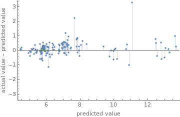
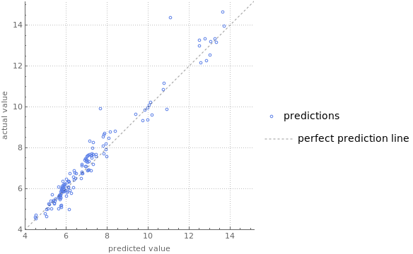
0.505262

If an investor is interested on making money from a predictor, the important thing to guess it's the direction of the price change. To see if the predictor can correctly guess the direction we construct a time series of the returns and look at their signs. Comparing between the actual time series and the predicted one there is a 65% success rate, meaning that the predictor gives an actual advantage over the a simple random walk guess.

Returns[x_,dt_]:= Drop[x,dt] - Take[x, {1,-(1+dt)}];
r1 = Returns[p[validationSet[[All,1]]], 1];
r2 = Returns[validationSet[[All,2]], 1];
N[Count[Sign[r1]-Sign[r2],0]/Length[r1]]

0.657343

Lastly we can pack all we have done in a manipulable predictor.

nercAreaRules = MapThread[#1->#2&, Transpose[nercAreaOfState]];
NercArea[state_]:= state /. nercAreaRules;

statealphabetarules = MapThread[#1->#2&, Transpose[statealphabetaparams]];
Statealphabeta[state_]:=state /. statealphabetarules;

Manipulate[
    GeoRegionValuePlot[
       Map[{#, p[{NercArea[#], Statealphabeta[#].{hdDays,cdDays}, coal, gas, gdp}]}&, states],
       ColorFunctionScaling->False,
       ColorFunction->(ColorData["Rainbow"][Log[#/6+0.2]]&)
    ],
    {{coal, 36, "Thermal coal price (Dollars per short ton)"}, 0, 100},
    {{gas, 4.29, "Natural gas price (Dollars per thousand cubic feet)"}, 0, 100},
    {{gdp, 3.7, "GDP (dollars per year)/10^10"}, 0, 100},
    {{hdDays, 300, "Heating degree days"}, 0, 1000, 1},
    {{cdDays, 0, "Cooling degree days"}, 0, 1000, 1}
]

Conclusions

Despite the apparent low success rate of 65.7% at trend prediction, this result is actually pretty amazing because in an efficient market there should be no possible way to predict the next direction of the price, since all the information about the expected value of the next price is encoded in the current price. But our predictor has apparently beaten the market with a small advantage. There is actually a trick to this, since in our validation set we have exact values of heating, cooling degree days and commodities prices, the predictor have a considerable advantage, but this just shows that in order to profit from electricity is just a matter of weather forecasting and some market speculation.

This project was made for the Wolfram Summer School 2017 to which I had the opportunity to attend. It was an amazing experience and it helped me a lot to improve my WL programming skills. It was also thrilling to meet all these talented people from around the world who also attended and did amazing things.

GitHub link

All the code and data can be found in my repo: https://github.com/CarlosManuelRodr/wss17

Data sources and references

Electricity prices by state and date: https://www.eia.gov/electricity/monthly/epmtablegrapher.php?t=epmt506_a

Natural gas price: https://www.eia.gov/dnav/ng/hist/n3035us3m.htm

Thermal coal price in the US (averaged): https://www.quandl.com/collections/markets/coal

High resolution NERC grid: https://public.opendatasoft.com/explore/dataset/nerc-regions/export/?flg=fr

Low resolution NERC grid: https://www.google.com/maps/d/viewer?mid=16rZqG5BrdTh3Lpkhmjs6oafMPaM&hl=en&ll=62.92523564759902%2C-125.22216709375002&z=4

Electricity price forecasting: A review of the state-of-the-art with a look into the future DOI: https://doi.org/10.1016/j.ijforecast.2014.08.008