Growth and spreading of topics on inSpireHEP

Brief and tentative description of the project carried out at the 2017 Wolfram Summer School.

The Mathematica notebook can be found here.

Goal of the project

The project has a twofold goal. Given a keyword representing a scientific topic (e.g., entanglement, gravitational waves, etc...), we compute the number of occurrences of the keyword that appears in the abstracts of papers in a given time interval and we study how papers about a specific topic are related to each other by analyzing the corresponding citations. In particular, we construct the citation graph associated to the topic and we display its time evolution.

Summary of the work

As a preliminary step, we download an updated snapshot of record metadata in JSON format containing information about one million of papers posted on inSpireHEP. After adjusting the database to our purposes, we collect the abstracts year by year. The first goal is reached by using the built-in function StringCount, which counts how many times the keyword appears in the abstracts within a given time interval. Then we chart the occurrences by using DateListPlot and few examples of keyword search are shown. The second goal is achieved by selecting those papers concerning the chosen topic and by associating each of these papers to their list of citations. We construct the corresponding citation graph and highlight the communities by centrality-based clustering criterion. We emphasize those papers whose position is relevant for the topology of the graph. Finally, we introduce a further time selection of papers (in addition to the topic selection) in order to display the time evolution of the graph.

Code explanation

First of all, we download the JSON file containing the record metadata (ID, title, abstract, authors, citations, references, publication date, etc...) from inSpireHEP website and save it as inSpire.json.

Then we import the file using the following line:

data = Part[
   Reap[
    Module[ {line, file = FileNameJoin[{NotebookDirectory[], "inSpire.json"}]}, 
     Quiet@Close[file];
     OpenRead[file];
     While[line =!= EndOfFile, line = ReadString[file, "\n"];
      Replace[line, _String :> Sow@Developer`ReadRawJSONString[line]]];
     ]
    ],
   2, 1
   ];

and save it

DumpSave["inSpire.mx", data]

The next step is to import the data

<< inSpire.mx

and clean it for our objectives. We will call the clean data pubdata.

For future convenience, we collect the abstracts year by year. We create an association between the creation date and the abstract of the paper and we organizeit in chronological order:

 abstractsWithDates =
  KeySort[#CreationDate -> #abstract & /@ Normal@pubdata // 
    Association] ;

We define a function to compare the year of two papers

equalDates[date2_][date1_] := 
 MatchQ[DateObject[DateValue[date1, "Year"]], 
  DateObject[DateValue[date2, "Year"]]]

and we select all those papers published in that given year:

abstractsAtYear[date_] := 
 KeySelect[abstractsWithDates, equalDates[date]]

abstractYearData[date_] := Values@abstractsAtYear[date] // StringRiffle

and finally we collect all the abstracts year by year from 1930 to 2017:

abstractText = 
  AssociationMap[abstractYearData, 
   DateRange[DateObject[{1930}], DateObject[{2017}], 
    Quantity[1, "Years"]]];

To avoid this evaluation every time, we save the abstracts collection in abstractText:

DumpSave[FileNameJoin@{NotebookDirectory[], 
   "abstractText.mx"}, abstractText]

Occurrences of keywords in abstract in a given time interval

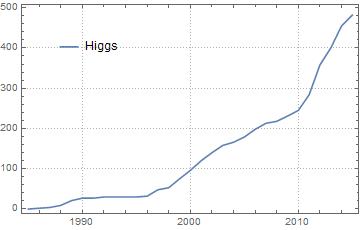
We are in a position to build a easy search engine for keywords in the abstracts. The user has two degrees of freedom in his search: the keyword and the time interval. The research engine is a useful analytical tool to show the trend of a topic in the time range. In the following, we present some representative examples.

We import all the abstracts

<< abstractText.mx

and define a function that counts how many times a given keyword appears in abstracts published in that year:

stringCountsAt[date_, words_] := StringCount[abstractText[date], words];
stringCountsAt[words_][date_] := stringCountsAt[date, words]

how many times a given keyword is counted up to that year:

stringCountUpTo[year_, words_, start_: Automatic] :=
 Map[
  stringCountsAt[words],
  Range[Replace[start, Automatic :> Min@Keys[abstractText]], 
   Replace[year, _Integer :> DateObject[{year}]], Quantity[1, "Years"]]
  ]

and how many occurrences in a time interval:

occurrences[word_String, dateStart_, 
  dateEnd_] := {#, stringCountUpTo[#, word] // Total} & /@ 
   Range[Replace[dateStart, _Integer :> DateObject[{dateStart}]], 
    Replace[dateEnd, _Integer :> DateObject[{dateEnd}]], 
    Quantity[1, "Years"]] // TimeSeries

We plot the occurrences of the keyword "Higgs" between 1985 and 2015

 DateListPlot[
 {occurrences["Higgs", 1985, 2015]}, 
 Joined -> True,
 PlotLegends -> Placed[{"Higgs"}, {0.2, 0.8}], 
 PlotTheme -> "Detailed",
 PlotRange -> Full
 ] 

Citations graph and its time evolution

In this section, we explain how to construct the citations graph for a given topic. The citations graph is an useful tool to visualize the relations between papers concerning the same topic and to highlight hidden properties among them. To meet this aim, we construct the citations graph of those papers about the "BMS group"

We select the papers with more than 20 citations:

citationsData = Select[
   pubdata,
   Length[#["citations"]] >= 20 &
   ];

and we define an association between ID and citations list, authors, abstracts and titles:

idWithCitations =
  #recid -> #citations & /@ Normal@citationsData // Association ;
idAuthor = #recid -> #authors & /@ Normal@citationsData // Association ;
idAbstract = #recid -> #abstract & /@ Normal@citationsData // Association ;
idTitle = #recid -> #title & /@ Normal@citationsData // Association ;
idCreationDate = #recid -> #CreationDate & /@ Normal@citationsData // 
   Association ;

We need to define other functions to compare dates and years:

compareDates[date1_, date2_] := 
  If[DateOverlapsQ[date1, date2], DateObject[{DateValue[date1, "Year"]}], 
   date1 < date2];
compareDates[date1_][date2_] := compareDates[date2, date1];
compareYears[date1_, date2_] := date1 <= date2;
compareYears[date1_Integer][date2_] := compareYears[date2, date1];
compareYears[date1_DateObject] := compareYears[DateValue[date1, "Year"]];

We select those papers containing the keyword in the abstract and define the association between the ID and the citations list:

idAbstractswithWord[words_String] := 
 Keys@Select[idAbstract, StringContainsQ[words]] 
idWithCitationsandTopic[words_String] := 
 Thread[# -> Lookup[idWithCitations, #]] &@idAbstractswithWord[words]

and plot the graph associated to that keyword (representing a concept/topic)

graphTopic = Graph[
   Thread /@ idWithCitationsandTopic["BMS group"] // Flatten,
   DirectedEdges -> False, 
   VertexStyle -> Red,
   VertexSize -> Automatic,
   ImageSize -> Automatic
   ];

We define the highly central vertices:

highlyCentral[graph_] := Pick[
  VertexList@graph,
  GreaterThan[10] /@ DegreeCentrality@graph
  ]

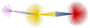
and display all the graph communities:

HighlightGraph[
 HighlightGraph[
  graphTopic,
  Map[Subgraph[graphTopic, #] &, 
   FindGraphCommunities[graphTopic, Method -> "Centrality"]]],
 Style[highlyCentral[graphTopic], Black], 
 ImageSize -> Large
 ]

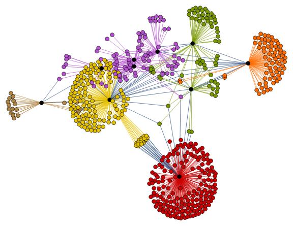
Within the whole set of papers about the "BMS group", we might select the most cited papers. The number of citations is usually a reliable bibliometric quantity to evaluate the scientific quality of a paper. In the graph above, we highlighted the graph communities in different colors and the papers with the highest degree of centrality in black. The latter set of papers is a subset of the most cited papers and they play an important role in the topological structure of the graph. In other words, among the most cited papers, we introduce the centrality-based clustering criterion to select the most "important" papers. As an example, the black vertex inside the yellow community is the so-called vertex cut. A vertex cut is that vertex whose removal renders the graph disconnected. In this respect, that paper connects different communities (i.e., different sub-topics) and it represents a seminal paper in the field because it has a non trivial topological position in the graph. In the case at hand, it is the paper by Ashtekar entitled "A unified treatment of null and spatial infinity in general relativity. I - Universal structure, asymptotic symmetries, and conserved quantities at spatial infinity".

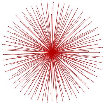
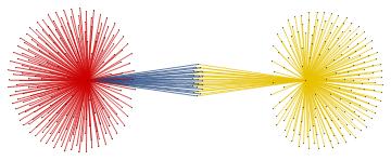
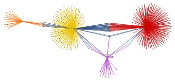
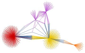
It is also interesting to visualize the time evolution of the graph during a given time interval. To achieve this result, we need snapshots of the citations graphs year by year. In other words, we need to further select papers by date, in addition to the first selection by topic, and construct the corresponding graph.

We therefore select those papers about a given topic published up to a given date:

idCreationYear = DateValue[#, "Year"] & /@ idCreationDate;

idAbstractswithDateTopic[date_, words_String] := 
 Intersection[Keys@Select[idCreationYear, compareYears[date]], 
  Keys@Select[idAbstract, StringContainsQ[words]]]
idCitations[date_, words_String] := 
 Thread[# -> Lookup[idWithCitations, #]] &@
  idAbstractswithDateTopic[date, words]

and compute the time evolution from 1978 to 2008

timeEvo = 
  idCitations[#, "BMS group"] & /@ 
   DateRange[DateObject[{1978}], DateObject[{2008}], 
    Quantity[1, "Years"]];

timeEvoPruned =
  With[{edges = Flatten[Thread /@ #]},
     Select[edges, Not@*MemberQ[Alternatives @@ #]] &@
      Pick[VertexList@edges, LessThan[0] /@ VertexDegree[edges]]
     ] & /@ timeEvo;

g = Table[
  Graph[timeEvoPruned[[i]], DirectedEdges -> False, 
   VertexStyle -> Red, VertexSize -> Small, 
   ImageSize -> Automatic], {i, 1, Length[timeEvoPruned]}];

CommunityConnectedGraph = Table[
   HighlightGraph[g[[i]], 
    Map[Subgraph[g[[i]], #] &, 
     FindGraphCommunities[g[[i]], Method -> "Centrality"]]], {i, 1, 
    Length[g]}];

ListAnimate[CommunityConnectedGraph]

For the "BMS group" the citations graph has the following growth:

Conclusion and future work

In this project, we defined a search engine that charts occurrences of any keyword in the abstracts of papers posted on inSpireHEP/arXiv.org and constructed the corresponding citation graph and highlighted the communities by centrality-based clustering criterion. We emphasized those papers about one specific chosen topic that play an important role in the structure of the citations graph, because of their high degree of centrality and not only because they are the most cited papers in the field. Finally, we displayed the time evolution of the graph.

Future directions of investigation require more complete database and a detailed analysis of the topological properties of the graph.