This is a summary of my findings regarding the set of Clausius-Clapeyron Relations that I researched during my time at the 2017 Wolfram High School Summer Camp. During the time that I worked on the project, I learned much about the implementation of the relations to physical systems and the Wolfram Language in general. Although there were some initial issues with creating the plot, I was able to create a successful interactive plot of the phase boundary in the end. The final project was a series of plots that can determine a phase boundary based on the manipulate functionality in the Wolfram program. Attached is the final project notebook that I created with all the code necessary for generating the plots.

The Clausius-Clapeyron Relations

The set of Clausius-Clapeyron differential equations relates the change of an external thermodynamic variable such as magnetic field or vapor pressure with respect to temperature. The solution curve is a phase boundary where the system changes its magnetic ordering state or matter phase as it crosses the boundary. A program was created which determines the general behavior of this phase boundary based on system variables such as entropy change (?S), latent heat (L), and volume change (?V) inputted as linear parameters of relative intensity. The program can be used to observe how these thermodynamic parameters affect the shape of a given phase boundary between two different physical states. Possible applications of this program are simulations of magnetic and matter phase transitions, enhanced analysis of experimental diagrams, and prediction of phase boundaries. Note that the program created can be used to determine the general shape and behavior of phase boundaries given an input ratio of the system's thermodynamic properties in units of relative intensity. However, the first few plots that I created are able to identify the overall shape of the phase boundary line rather than its exact coordinates.

Magnetic Phase Transitions

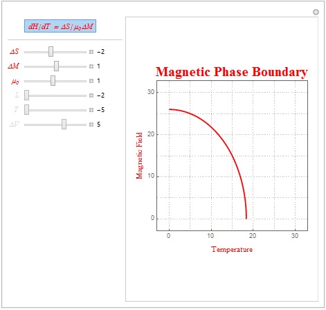
The first form Clausius-Clapeyron relation that was explored was for magnetic systems. This relation is written as dH/dT = ?S/(µ?M) where ?S is the entropy change of the system, µ is the magnetic permeability of the system, and ?M is the total change in magnetization. If we approximate ?S and ?M as linear functions dependent on T (temperature) and H (magnetic field), respectively, then we will be able to create a phase boundary above which the system becomes paramagnetic, or disordered. Below is the code that I used to create the plot.

Manipulate[
 f[1, x_, y_] := (a*x)/ (\[Mu]*(y*m));

 VectorPlot[{1, f[p, x, y]}, {x, 0, 30}, {y, 0, 30}, 
         FrameLabel -> {Style["Temperature", 12, 
     FontFamily -> "Times", Red], 
    Style["Magnetic Field", 12, FontFamily -> "Times", Red]}, 
  AxesStyle -> Red, VectorScale -> {.05, Automatic, None}, 
  ImageSize -> {280, 430}, VectorStyle -> Blue, 
  PlotLabel -> 
   Style["Magnetic Phase Boundary", 22, FontFamily -> "Times", Red, 
    Bold], StreamStyle -> {Red, Arrowheads[0]}, StreamPoints -> 1, 
  VectorPoints -> 0, StreamScale -> Full, PlotTheme -> "Business", 
  StreamScale -> Full]

Some interesting linear parameters are ?S = -2, ?M = 1, and µ=1 (as shown in the plot below). These parameters are characteristic of an antiferromagnetic system as the system has a negative ?S. Note that below the red line the magnetic alignment is antiferromagnetic but above the red line the magnetic alignment is paramagnetic. Another set of interesting parameters, representative of a diamagnetic material (magnetic permeability less than 1) is ?S = -2, ?M = 2, and µ=.1.

Pressure Phase Transitions

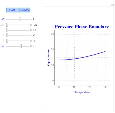
Two common forms of the Clausius-Clapeyron Relation are dP/dT = L/(T?V) and dP/dT = (?S/?V). The shape of these boundaries was created using the same technique outlined above. In these relations, L represents latent heat, ?S represents entropy change, T is the temperature of the system, and ?V is the volume change of the system.

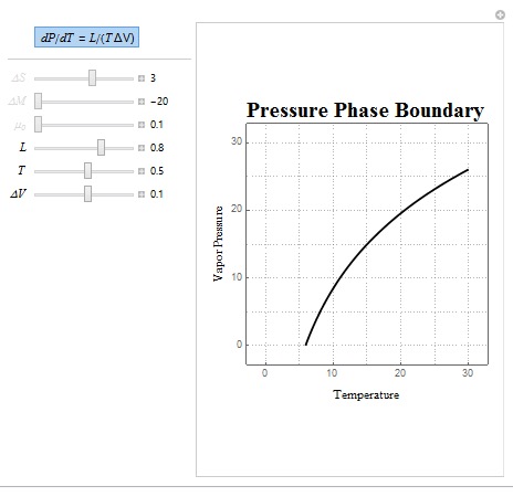
Shown above is a sample matter phase diagram plot which allows the user to manipulate the ratio of latent heat (L), temperature, and volume change (?V) where the latter two are approximated using linear functions. Some interesting parameters to use are negative ?V values as inputting these parameters show how the phase boundary behaves when the system is compressed.

Shown below is another sample diagram which uses the parameters ?S and ?V instead.

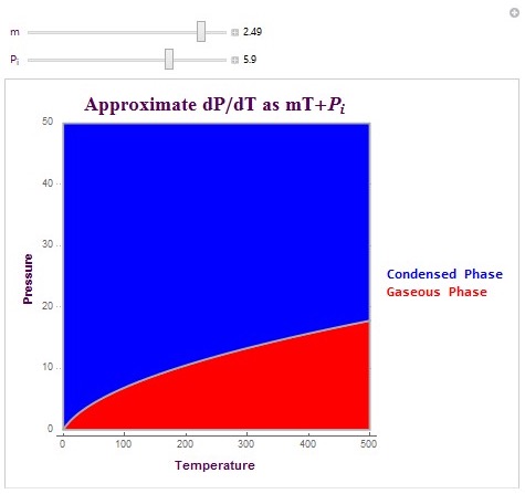
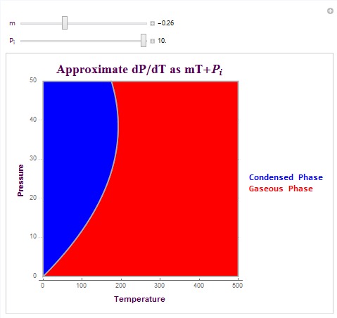
Another type of plot which I created is able to create the exact phase boundary for matter phase transitions. This plot is able to create the actual pressure phase line by allowing the user to linearly approximate dP/dT (change in pressure versus temperature). It then integrates this linear equation to plot the matter phase boundary in terms of vapor pressure. The equation that I used here was dP/dT = mT+ Pi. In this equation, m is the linear change parameter and Pi is the initial pressure condition. These parameters can be determined experimentally or they can be predicted parameters. The following is the code used to create the plot and its output (with specific conditions).

Style["dP/dT = mT+\!\(\*SubscriptBox[\(P\), \(i\)]\)", Purple, 
    Bold] -> 
   Manipulate[
    Show[{RegionPlot[
       p > Evaluate[(Integrate[(m s + b) , s] /. s -> v)], {p, 0, 
        500}, {v, 0, 50}, 
       PlotLabel -> 
        Style["Approximate dP/dT as mT+\!\(\*SubscriptBox[\(P\), \
\(i\)]\)", FontFamily -> "Times", Bold, 20, Darker@Purple], 
       PlotStyle -> Red, 
       PlotLegends -> 
        Style["Condensed Phase", Blue, FontFamily -> "Times", Bold, 
         14], FrameLabel -> {Style["Temperature", Bold, 12, 
          Darker@Purple], Style["Pressure", Bold, 12, Darker@Purple]},
        PlotTheme -> "Business", 
       BoundaryStyle -> {Thick, Darker@White}], 
      RegionPlot[
       p < Evaluate[(Integrate[(m s + b) , s] /. s -> v)], {p, 0, 
        500}, {v, 0, 50}, PlotStyle -> Blue, 
       BoundaryStyle -> {Thick, Darker@White}, 
       PlotLegends -> 
        Style["Gaseous Phase", Red, FontFamily -> "Times", Bold, 14], 
       PlotTheme -> "Business"]}],

    {{m, 2, Style["m", Darker[Purple]]}, -2, 3, 
     Appearance -> "Labeled"},
    {{b, 1, 
      Style["\!\(\*SubscriptBox[\(P\), \(i\)]\)", 
       Darker[Purple]]}, -5, 10, Appearance -> "Labeled"}
    ]

  }]

These are two matter phase diagram plots with interesting conditions that affect the concavity of the phase boundary. Note that in the second diagram there exists a possible triple point at which the system switches to a liquid phase rather than remaining in its gaseous state (as shown in red). The possible triple point is (100,15) in temperature-pressure coordinates.

Conclusion

Four different forms of the Clausius-Clapeyron equation were used in the creation of these diagrams which plot the general behavior of the phase boundary. The first form of the Clausius-Clapeyron equation used was for magnetic systems. In magnetic systems, the phase boundary determined by the Clausius Clapeyron equation marks the transition between an ordered ferromagnetic or antiferromagnetic state below the phase line to a disordered paramagnetic state above the phase line in magnetic materials. This phase boundary is in expressed as a scalar applied magnetic field as a function of temperature. The other three forms of the Clausius-Clapeyron equations used in this program are for matter phase change systems. In these forms, the phase boundary marks the transition between a gaseous state below the phase line to a condensed matter state above the phase line. These phase boundaries are expressed in terms of a scalar vapor pressure as a function of temperature.

Further work could further the generalization of the Clausius-Clapeyron Relation to magnetic and similar thermodynamic systems and use other approximation techniques. Ultimately, programs like the one created here should be used in the experimental process when generating thermodynamic data and phase diagrams of real-world systems and materials.

Attachments: