Description
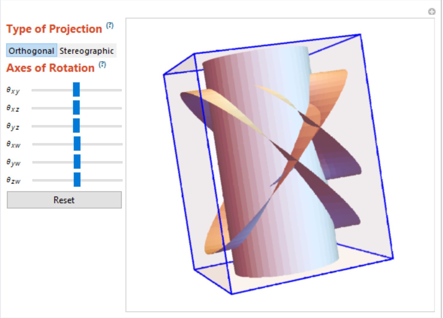
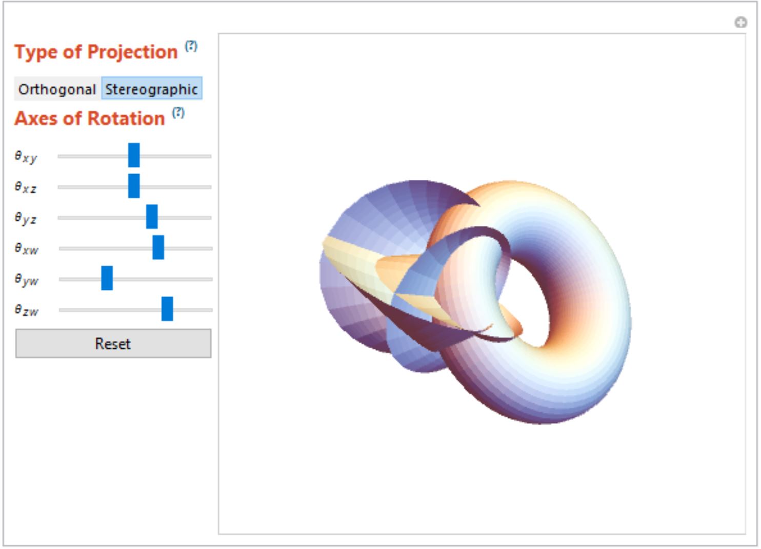
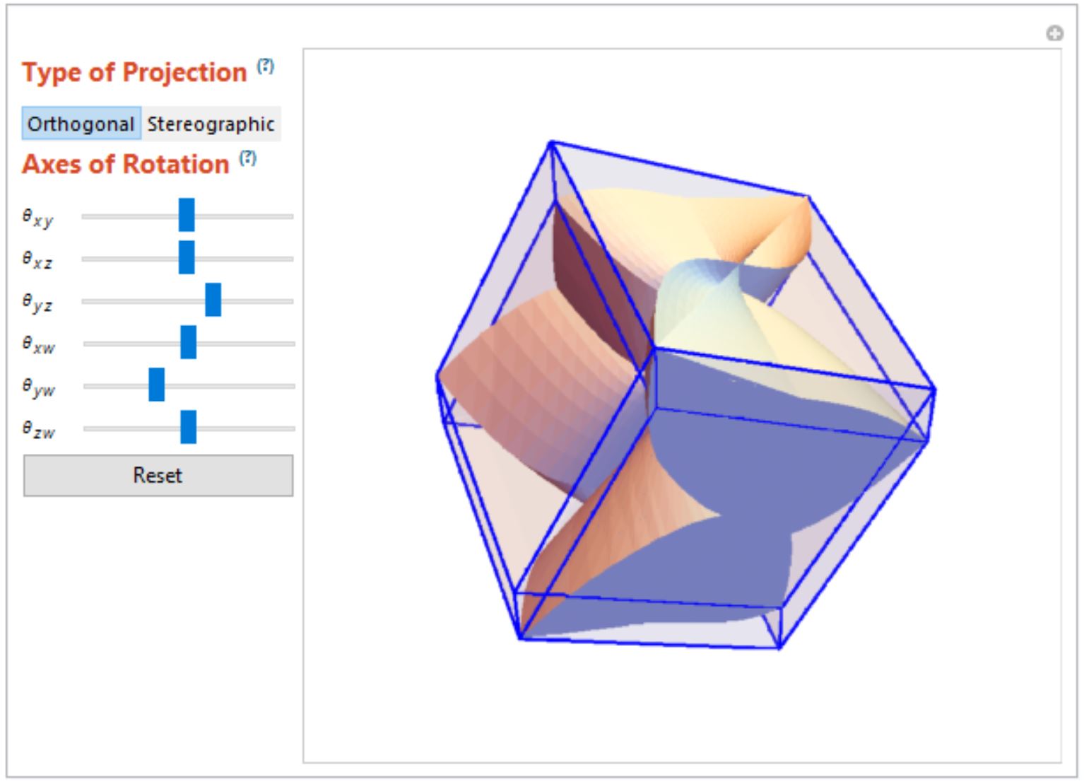
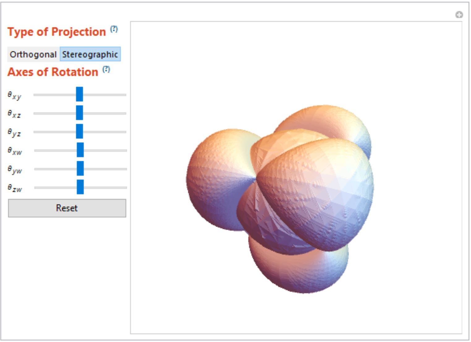
ParametricPlot4D projects a 4D parameterization either orthogonally or stereographically to make a 3D shadow and uses Graphics3D to render it. In the orthogonal projection case, the function displays the bounding tesseract, which is analogous to Plot3D's bounding rectangular prism and Plot2D's bounding rectangle.
Initialization
Projections
Below are the formulas for the orthogonal and stereographic projections:
orthogonalProjection[{x_, y_, z_, w_}] := {x, y, z}
orthogonalProjection[Polygon[list_]] :=
 Polygon[Most /@ list]
orthogonalProjection[list_List] :=
 orthogonalProjection /@ list

stereographicProjection[{x1_, y1_, z1_, w1_}] :=
  Block[{x, y, z, w},
   {x, y, z, w} = Normalize[{x1, y1, z1, w1}];
   {x/(1 - w), y/(1 - w), z/(1 - w)}
   ];
The orthogonal projection is equipped with rotating a list of polygons because the orthogonal bounding tesseract has to be updated as the orthogonal projection is manipulated.
Rotations
Below is code for rotations about the 6 planes in 4D space:
rotate4DPoint[{x_, y_, z_,
   w_}, {?1_, ?2_, ?3_, ?4_, ?5_, \
?6_}] := Block[{c1, c2, c3, c4, c5, c6, s1, s2, s3, s4, s5, s6},
  {c1, c2, c3, c4, c5, c6} =
   Cos[{?1, ?2, ?3, ?4, ?5, \
?6}];
  {s1, s2, s3, s4, s5, s6} =
   Sin[{?1, ?2, ?3, ?4, ?5, \
?6}];
  {
    {c1 c2 c3, -c4 c5 s1 - c1 (c5 s2 s4 + c2 s3 s5),
     s1 (c6 s4 + c4 s5 s6) - c1 (c4 c6 s2 + (c2 c5 s3 - s2 s4 s5) s6),
      s1 (c4 c6 s5 - s4 s6) +
      c1 (-c2 c5 c6 s3 + s2 (c6 s4 s5 + c4 s6))},
    {c2 c3 s1,
     c1 c4 c5 - s1 (c5 s2 s4 + c2 s3 s5), -c1 c6 s4 +
      s1 (-c2 c5 s3 + s2 s4 s5) s6 -
      c4 (c6 s1 s2 + c1 s5 s6), -c2 c5 c6 s1 s3 +
      s1 s2 (c6 s4 s5 + c4 s6) + c1 (-c4 c6 s5 + s4 s6)},
    {c3 s2, c2 c5 s4 - s2 s3 s5,
     c2 c4 c6 - (c5 s2 s3 + c2 s4 s5) s6, -c5 c6 s2 s3 -
      c2 (c6 s4 s5 + c4 s6)},
    {s3, c3 s5, c3 c5 s6, c3 c5 c6}
    }.{x, y, z, w}
  ]
The rotatePolygons function is necessary to dynamically update the bounding tesseract.
Tesseract Coordinate Bounds
Below is a function to generate coordinate bounds for the dimensions of the bounding tesseract of a surface:
tesseractBounds[
  expr_ /; TensorRank[expr] == 1, {u_, uMin_, uMax_}, {v_, vMin_,
   vMax_}] :=
 With[{su = $steps, sv = $steps},
  CoordinateBounds@
   Table[N[expr], {u, uMin, uMax, (uMax - uMin)/su}, {v, vMin,
     vMax, (vMax - vMin)/sv}]
  ]
In total, there are 6 functions because each pair of functions represents finding bounds on one or a list of curves, surfaces, or volumes. Once we have these bounds, we generate the tesseract faces for Graphics3D to render, as shown below:
tcells = {{1, 5, 13, 9}, {2, 6, 14, 10}, {3, 7, 15, 11}, {4, 8, 16,
    12}, {1, 3, 11, 9}, {2, 4, 12, 10}, {5, 7, 15, 13}, {6, 8, 16,
    14}, {1, 2, 10, 9}, {3, 4, 12, 11}, {5, 6, 14, 13}, {7, 8, 16,
    15}, {1, 3, 7, 5}, {2, 4, 8, 6}, {9, 11, 15, 13}, {10, 12, 16,
    14}, {1, 2, 6, 5}, {3, 4, 8, 7}, {9, 10, 14, 13}, {11, 12, 16,
    15}, {1, 2, 4, 3}, {5, 6, 8, 7}, {9, 10, 12, 11}, {13, 14, 16,
    15}};

tesseractFaces[bds_] := With[{tups = Tuples[bds]},
  tups[[#]] & /@ tcells
  ]
These $24=\dbinom{4}{2} \cdot 2^{4-2}$ faces were generated through a function that lists coordinates for all $j$-D cube subsets of a $i$-D cube. It first iterates through the $\dbinom{i}{j}$ permutations of $j$ $1$'s and $i-j$ $0$'s, then toggles the $j$ $1$'s to become Tuples[{min, max}, j] in each permutation to build a $j-D$ hypercube subset, and finally toggles the $i-j$ 0's to become Tuples[{min, max}, i-j] generate all hypercube subsets for that permutation. This is essentially an implementation of the $\dbinom{i}{j} \cdot 2^{i-j}$ hypercube subset formula.
Small Pieces of Curves, Surfaces, and Volumes
Below are functions that make the tiny elements of a curve, surface, or volume, respectively:
dLs[expr_, {u_, umin_, umax_}, rotation_, proj_] :=
 With[{su = $steps},
  grid = Table[
    proj[rotate4DPoint[N[expr], rotation]], {u, umin,
     umax, (umax - umin)/su}];
  partitioned = Partition[grid, {2}, 1];
  Line[Flatten[partitioned, {2}][[1]]]
  ]

dAs[expr_, {u_, umin_, umax_}, {v_, vmin_, vmax_}, rotation_, proj_] :=
 With[{su = $steps, sv = $steps},
  grid = Table[
    proj[rotate4DPoint[N[expr], rotation]], {u, umin,
     umax, (umax - umin)/su}, {v, vmin, vmax, (vmax - vmin)/sv}];
  partitioned = Partition[grid, {2, 2}, 1];
  Flatten[
   Replace[partitioned, {{a_, b_}, {c_, d_}} :>
     Polygon[{a, b, d, c}], {2}]]
  ]

makeCube[cube_] :=
 GraphicsComplex[Flatten[cube, 2],
  Polygon[{{5, 1, 2}, {1, 4, 2}, {1, 5, 3}, {5, 7, 3}, {5, 6, 8}, {6,
     4, 8}, {4, 6, 2}, {6, 5, 2}, {7, 4, 3}, {4, 1, 3}, {4, 7, 8}, {7,
      5, 8}}]]
dVs[expr_, {u_, umin_, umax_}, {v_, vmin_, vmax_}, {w_, wmin_, wmax_},
   rotation_, proj_] :=
 With[{su = $steps, sv = $steps, sw = $steps},
  grid = Table[
    proj[rotate4DPoint[N[expr], rotation]], {u, umin,
     umax, (umax - umin)/su}, {v, vmin, vmax, (vmax - vmin)/sv}, {w,
     wmin, wmax, (wmax - wmin)/sw}];
  partitioned = Partition[grid, {2, 2, 2}, 1];
  Flatten@Map[makeCube, partitioned, {3}]
  ]
The particularly interesting case is the dVs; the 6 faces of each dV are mapped to 12 triangles, which can all be treated the same way the dAs are. Of course, the sheer number of polygons makes this computationally expensive, and optimizations would be appreciated.
Surface Parameterizations
Below are some default surface parameterizations:
torus3[R_, P_][u_, v_] := {R Cos[u], R Sin[u], P Cos[v], P Sin[v]}
sphere3[R_, ?_][?_, ?_] :=
 R*{Cos[?], Sin[?] Cos[?], Sin[?] Sin[?] Cos[?],
   Sin[?] Sin[?] Sin[?]}
kleinSurface[P_, e_][u_, v_] := {
  -P (-2 + Abs[-1 + P]) Sin[u] (1 + e Sin[v]),
  P (-2 + Abs[-1 + P]) Cos[u] (1 + e Sin[v]),
  -(((-2 + Abs[-1 + P]) (Cos[v] Sin[u/2] + Cos[u/2] Sin[2 v]))/P),
  ((-2 + Abs[-1 + P]) (Cos[u/2] Cos[v] - Sin[u/2] Sin[2 v]))/P
  }
hyperCone[vx_, vy_, vz_][t_, s_][?_, ?_] := {vx t +
   t s Cos[?] Cos[?],
  vy t + t s Cos[?] Sin[?], vz t + t s Sin[?], t}
Plotting
Below is my ParametricPlot4D code for one surface:
ParametricPlot4D[
  expr_ /; TensorRank[expr] == 1, {u_, uMin_, uMax_}, {v_, vMin_,
   vMax_}, opts : OptionsPattern[]] :=
 Manipulate[

  If[SameQ[proj, orthogonalProjection],

   Graphics3D[
    {
     {EdgeForm[{Thick, Blue}], {Opacity[0.1],
       proj /@ rotatePolygons[
         Polygon /@
          tesseractFaces[
           tesseractBounds[
            N[expr], {u, uMin, uMax}, {v, vMin,
             vMax}]], {?1, ?2, ?3, ?4, \
?5, ?6}]}}, {EdgeForm[
       OptionValue[EdgeForm]], {dAs[
        N[expr], {u, uMin, uMax}, {v, vMin,
         vMax}, {?1, ?2, ?3, ?4, \
?5, ?6}, proj]}}
     }, Boxed -> OptionValue[Boxed]],

   Graphics3D[
    {EdgeForm[
      OptionValue[EdgeForm]], {dAs[
       N[expr], {u, uMin, uMax}, {v, vMin,
        vMax}, {?1, ?2, ?3, ?4, \
?5, ?6}, proj]}},
    Boxed -> OptionValue[Boxed], PlotRange -> OptionValue[PlotRange]]

   ],
  {proj, {orthogonalProjection, stereographicProjection},
   ControlType -> None},
  {{?1, 0}, -2 Pi, 2 Pi, ControlType -> None},
  {{?2, 0}, -2 Pi, 2 Pi, ControlType -> None},
  {{?3, 0}, -2 Pi, 2 Pi, ControlType -> None},
  {{?4, 0}, -2 Pi, 2 Pi, ControlType -> None},
  {{?5, 0}, -2 Pi, 2 Pi, ControlType -> None},
  {{?6, 0}, -2 Pi, 2 Pi, ControlType -> None},

  Row[{
    Style[
     "Type of Projection", {15, Bold,
      RGBColor[214/255, 74/255, 13/85]}],
    Spacer[5],
    Column[{Tooltip[
       Style["(?)", {10, Bold, RGBColor[4/85, 6/17, 43/85]}],
       Style[
        "Orthogonal Projection transforms {x,y,z,w} into {x,y,z}\n\
Stereographic Projection transforms {x,y,z,w} into a normalized \
{x/(1-w),y/(1-w),z/(1-w)}",
        {12}],
       TooltipDelay -> 0.1],
      ""}]
    }],

  Row[{SetterBar[
     Dynamic[proj], {orthogonalProjection -> "Orthogonal",
      stereographicProjection -> "Stereographic"}]}],
  Row[{
    Style[
     "Axes of Rotation", {15, Bold, RGBColor[214/255, 74/255, 13/85]}],
    Spacer[5],
    Column[{Tooltip[
       Style["(?)", {10, Bold, RGBColor[4/85, 6/17, 43/85]}],
       Style[
        "Each of these sliders (ranging from -2? to 2?) controls a rotation in the hyperplane\nspanned by the Euclidean basis
vectors. Since this is a projection of R^4, the axes x, y, z,\nand w \
correspond to the vectors {1,0,0,0\
}, {0,1,0,0}, \
{0,0,1,0}, and \
{0,0,0,1}, \nrespectively.",
        {12}],
       TooltipDelay -> 0.1],
      ""}]
    }],

  Row[{Style[Subscript["?",
     Row[{Style["x", Italic], "\[InvisibleSpace]",
       Style["y", Italic]}]], 9], Spacer[15],
    Slider[Dynamic[?1], {-2.0 Pi, 2.0 Pi},
     ImageSize -> {120, 20}]}],
  Row[{Style[Subscript["?",
     Row[{Style["x", Italic], "\[InvisibleSpace]",
       Style["z", Italic]}]], 9], Spacer[15],
    Slider[Dynamic[?2], {-2.0 Pi, 2.0 Pi},
     ImageSize -> {120, 20}]}],
  Row[{Style[Subscript["?",
     Row[{Style["y", Italic], "\[InvisibleSpace]",
       Style["z", Italic]}]], 9], Spacer[15],
    Slider[Dynamic[?3], {-2.0 Pi, 2.0 Pi},
     ImageSize -> {120, 20}]}],
  Row[{Style[Subscript["?",
     Row[{Style["x", Italic], "\[InvisibleSpace]",
       Style["w", Italic]}]], 9], Spacer[15],
    Slider[Dynamic[?4], {-2.0 Pi, 2.0 Pi},
     ImageSize -> {120, 20}]}],
  Row[{Style[Subscript["?",
     Row[{Style["y", Italic], "\[InvisibleSpace]",
       Style["w", Italic]}]], 9], Spacer[15],
    Slider[Dynamic[?5], {-2.0 Pi, 2.0 Pi},
     ImageSize -> {120, 20}]}],
  Row[{Style[Subscript["?",
     Row[{Style["z", Italic], "\[InvisibleSpace]",
       Style["w", Italic]}]], 9], Spacer[15],
    Slider[Dynamic[?6], {-2.0 Pi, 2.0 Pi},
     ImageSize -> {120, 20}]}],

  Button["Reset",
   {?1, ?2, ?3, ?4, ?5, ?6} \
= {0.0, 0.0, 0.0, 0.0, 0.0, 0.0};
   ]
  ]
The important parts to note are that the 6 rotation angles can be manipulated at the user's preference, and a lot of functions are necessary to render the bounding tesseract due to the fact that it has to be dynamically updated as the 6 rotation angles are manipulated.
Example Plots
ParametricPlot4D[{hyperCone[0.0, 0.0, 0.0][1.5, 1.][u, v], hyperCone[0.5, 0.5, 0.5][1., 1.][u, v], torus3[1., 2.][u, v]}, {u, -Pi, Pi}, {v, -Pi, Pi}]

ParametricPlot4D[{torus3[1, 2][a, b], kleinSurface[1.5, .5][a, b], hyperCone[0.5, 0.5, 0.5][1., 1.5][a, b]}, {a, -Pi, Pi}, {b, -Pi, Pi}, PlotRange -> All]

ParametricPlot4D[{{r^3, s^3, t^3, r s t}, {r, s, t, r s t}}, {r, -1., 1.}, {s, -1., 1.}, {t, -1., 1.}]

ParametricPlot4D[{{r^3, s^3, t^3, r s t}, {r, s, t, r s t}}, {r, -1., 1.}, {s, -1., 1.}, {t, -1., 1.}]

Conclusion
ParametricPlot4D was very successful in rendering curves and surfaces because the number of dLs and dAs was not overwhelmingly large. However, the function was extremely slow in rendering volumes due to the sheer number of dVs and dAs, as one dV corresponded to 12 dAs. Further work could be done in improving volume rendering and creating a general Plot4D function.
 Attachments: