Message Boards Message Boards

0
|
3278 Views
|
4 Replies
|
3 Total Likes
View groups...
Share
Share this post:

[?] Resolve singularity in ODE under DSolve?

Posted 7 years ago

Hi all, I am fairly new to Mathematica, and try to solve some of my ODEs using DSolve. I know that when x = -1, and 1, I have an undefined derivative. So I am just planning to solve between -1+eps and 1-eps, where eps = 0.0001. However, the following code enters some calculation loop and never finished the calculation. I have solved the same equation in MATLAB, and pretty sure it is solvable, but would like to use DSolve for some other purposes. Here is my code. Any help would be appreciated!

ClearAll["Global`*"];
w = 0.7
q = 0.5*w*(1 - x^2)
kappa = 1.469
sol = DSolve[{y'[x] == (560*x^0.5*q - 64*x^4 + 
       6*w^(7/8)*(72*kappa - 77)*x*q*(-w*x))/(3*
       w^(7/8)*(96*kappa - 77)*q^2), y[-0.99999] == 0.00001}, 
  y[x], {x, -0.99999, 0.99999}]
POSTED BY: Kai D
4 Replies
Posted 7 years ago

Sorry, I think I made a typo in my equation. I must apologize for this. I have attached the new one. But it still seems unsovlable. My equation actually is following:

ClearAll["Global`*"];
w = 0.7
q = 0.5*w*(1 - x^2)
kappa = 1.469
sol = DSolve[{y'[x] == (560*y[x]^0.5*q - 64*y[x]^4 + 
       6*w^(7/8)*(72*kappa - 77)*x*q*(-w*y[x]))/(3*
       w^(7/8)*(96*kappa - 77)*q^2), y[-0.99999] == 0.00001}, 
  y[x], {x, -0.99999, 0.99999}]

I actually solved this using MATLAB ode113, but because I would like do more coupling and more complicated boundary conditions, so I decided to give it a try in Mathematica.

Here is the link to my MATLAB if you are interested in, it is the exactly the same equation? https://www.mathworks.com/matlabcentral/answers/349482-singular-problem-for-bvp4c

POSTED BY: Kai D

DSolve is a symbolic solver and did not find it a solution.We have to use a numeric solver NDSolve.

w = 0.7;
q = 0.5*w*(1 - x^2);
kappa = 1.469;
sol = With[{eps = 10^-5}, NDSolve[{y'[x] == (560*y[x]^0.5*q - 64*y[x]^4 + 
6*w^(7/8)*(72*kappa - 77)*x*q*(-w*y[x]))/(3*w^(7/8)*(96*kappa - 77)*q^2), y[-1 + eps] == eps}, y, {x, -1 + eps, 1 - eps}]];
Plot[{Evaluate[y[x] /. sol]}, {x, -0.999, 0.999}, PlotLabels -> "solution"]

enter image description here

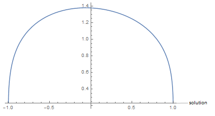
with High Precision:

  w = 7/10;
  q = 1/2*w*(1 - x^2);
  kappa = 1469/1000;
  sol = With[{eps = 10^-18}, 
    NDSolve[{y'[
        x] == (560*y[x]^(1/2)*q - 64*y[x]^4 + 
          6*w^(7/8)*(72*kappa - 77)*x*q*(-w*y[x]))/(3*
          w^(7/8)*(96*kappa - 77)*q^2), y[-1 + eps] == eps}, 
     y, {x, -1 + eps, 1 - eps}, WorkingPrecision -> 29, 
     MaxSteps -> Infinity, Method -> "ExplicitRungeKutta"]]

eps = 10^-18;
Plot[{Evaluate[y[x] /. sol]}, {x, -1 + eps, 1 - eps}, PlotLabels -> "solution"]
y[x] /. sol[[1]] /. x -> {0, -1 + eps, 1 - eps}(*in points x=0,-1,1*)
(* {1.3782772692251147769791113250, 0.*10^-18, 0.0000120776893357} *)
POSTED BY: Mariusz Iwaniuk
Posted 7 years ago

Thank you. This is exactly what I expect!

POSTED BY: Kai D

Well, if we solve equation I have:

y[x]=something+Constans

then putting yours boundary conditions y[-1] = 0 we have 0 = Infinity + Constans then: Constans = - infinity

  y[x]=something - infinity

In my opinion,is no solutions.

Code:

w = 7/10;
q = 1/2*w*(1 - x^2);
kappa = Rationalize[1.469, 0];
eq = (560*x^(1/2)*q - 64*x^4 + 6*w^(7/8)*(72*kappa - 77)*x*q*(-w*x))/(3*w^(7/8)*(96*kappa - 77)*q^2) // Expand
Y[X] = Integrate[#, x] & /@ (eq)
Limit[Y[X], x -> -1]
POSTED BY: Mariusz Iwaniuk
Reply to this discussion
Community posts can be styled and formatted using the Markdown syntax.
Reply Preview
Attachments
Remove
or Discard

Group Abstract Group Abstract