Hi All,
I would like to solve two ODEs coupled together using NDSolve, please see below for my code. Basically, I have two variables, y'[x] and g'[x] (not g''x]). The reason why I formulate my ODE using g''[x] is that I have integral boundary condition on g'[x], so I use the trick from [here to reformulate my equation. I will be happy to provide an original form of the equation if there is a question that is related to this part.
My problem is Mathematica complaints about "Infinite expression encountered" for my second equation(g''[x]) part. My guess is that in the denominator of this equation, It has y[x] term which equals to 0 at left boundary. Even though I tried to avoid this by calculating y[-1+eps]=eps, It appears to still have this issue.
ClearAll["Global`*"];
w = 0.7;
q = 0.5*w*(1 - x^2);
kappa = 1.469;
sol = With[{eps = 10^-5}, NDSolve[{
y'[x] == (560*y[x]^0.5*q - 64*y[x]^4 + 6*w^(7/8)*(72*kappa - 77)*x*q*(-w*y[x]))/(3*w^(7/8)*(96*kappa - 77)*q^2),
g''[x] == (2695*y[x]^0.5*q - (864*kappa - 385)*y[x]^4 - 693*w^(7/8)*kappa*y[x]*q*(-w*x))/(9*(96*kappa - 77)*y[x]^3),
y[-1 + eps] == eps,
g[1 - eps] - g[-1 + eps] == 0,
g'[0] == 0}, {y[x], g'[x]},
{x, -1 + 0.001, 1 - 0.001}]];
Methods that I have tried is to give initial condition to Mathematica like below. (As suggested by here). However, I encountered error " Initial conditions should be specified at a single point."
ClearAll["Global`*"];
w = 0.7;
q = 0.5*w*(1 - x^2);
kappa = 1.469;
sol = With[{eps = 10^-5}, NDSolve[{
     y'[x] == (560*y[x]^0.5*q - 64*y[x]^4 + 6*w^(7/8)*(72*kappa - 77)*x*q*(-w*y[x]))/(3*w^(7/8)*(96*kappa - 77)*q^2),
     g''[x] == (2695*y[x]^0.5*q - (864*kappa - 385)*y[x]^4 - 693*w^(7/8)*kappa*y[x]*q*(-w*x))/(9*(96*kappa - 77)*y[x]^3),
     y[-1 + eps] == eps, g[1 - eps] - g[-1 + eps] == 0,
     g'[0] == 0}, {y[x], g'[x]},
    {x, -1 + 0.001, 1 - 0.001},
    Method -> {"Shooting",
      "StartingInitialConditions" -> {y[-1 + eps] == eps,
        g'[eps] == 0}}]];
Any help will be greatly appreciated! Also, I have a related question: Right now, I have 2 ODEs, but I am planning to add transient terms d/dt for each variable I am solving at here. Let's assume Mathematica could solve these ODEs. Is it possible to solve the transient PDEs? It will be a transient 1D problem, and from the NDSolve documentation, it seems that Mathematica should have capabilities to solve it.
------------------------Update for the original equation-----------------
My x range is from -1 to 1. Here are equations that I would like to solve
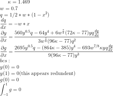
I also noticed here that this problem can be formulated as an optimization problem. However, I am having difficulty in this line of code on that link:
sol2[bc2_, {xmin_, xmax_}] :=
 NDSolveValue[{y''[x] - y[x] == (x^2), y'[0] == bc2, y[0] == 1}, y, {x, xmin, xmax}];
int[bc2_?NumericQ] := NIntegrate[sol2[bc2, {0, 2}][x], {x, 0, 2}];
**y2 = sol2[NMinimize[(int[bc2V] - 5)^2, bc2V][[-1, -1, -1]], {-3, 3}]**
Plot[{y1[x], y2[x]}, {x, -3, 3}]
I don't know what does [-1,-1,-1] has to do with the original problem or formulation.


