Original Question

There used to be a question about a manual implementation of the Adams-Bashforth method of numerically integrating an ODE. The code looked like it had be translate from C. I started to write up a more functional-programming to the problem. Well, why not share what I had done? Presumably the purpose of the writing the solver is educational. I will keep the design simple. For a more robust approach, I would recommend working within the NDSolve framework.

The original code looked something like this:

MyAdamBashforth[F_, h_, t_, y_][{t0_, y0_}] := 
 Module[{j, p, m, a, F0, F1, F2},
  m = 8;
  a = 0;
  t[0] = t0;
  y[0] = y0;
  For[j = 0, j <= 1, j++,
   t[j + 1] = t[j] + h;
   y[j + 1] = y[j] + h*F[t[j], y[j]];
   ];
  F0 = F[t[0], y[0]];
  F1 = F[t[1], y[1]];
  F2 = F[t[2], y[2]];
  For[j = 2, j <= m, j++,
   p = y[j] + h/12 (5 F0 - 16 F1 + 23 F2);
   t[j + 1] = t[j] + h;
   y[j + 1] = p;
   F0 = F1;
   F1 = F2;
   F2 = F[t[j + 1], y[j + 1]];
   ];
  ]

The solver was used in a way like this:

Clear[F, y, t, h];
F[t_, y_] := t + y;
MyAdamBashforth[F, 0.5, t, y][{0., 1.}]
MyData3 = Table[{t[j], y[j]}, {j, 0, 8}]

(*  {{0., 1.}, {0.5, 1.5}, {1., 2.5}, {1.5, 4.72917}, {2., 8.78212},
     {2.5, 15.6914}, {3., 27.2344}, {3.5, 46.3278}, {4., 77.713}}  *)

Design choices

In general, the (discrete) solution of an ODE $x'(t) = \text{RHS}(t, x(t))$ over $a \le t \le b$ consists of step data

$$ t_j, x_j, x'_j,\dots \quad \text{for}\ j = 0, 1, \dots, n\,,$$

where $t_0=a$, $t_n=b$, and the number of derivative values $x'_j, x''_j,\dots$ store for each step, if any, may depend on the method. For a first or higher order ODE, $x'_j$ is calculated anyway and may be used for cubic Hermite interpolation between the steps. In a multistep method, the $j+1$ step is computed from some number of the previous steps; single-step methods use only step $j$. The Adams-Bashforth (AB) method is a linear $s$-step method that uses only the values of $x'$ from the previous $s$ steps.

Input: Representation of the problem

Following the original question, the ODE will be specified by a function rhs that represents the first-order equation x'[t] == rhs[t, x[t]]. The initial condition (IC) is simply two numbers t0, x0, representing x[t0] == x0. Also we will require a final time t1, a step size h, and the step order s.

Output data structure

The output will be a list of the step data. The data for a step consists of $t, x, p=x'$. Neither the time $t$ nor the derivative $p$ are strictly necessary to keep, but they can be convenient to keep for the sake of interpolation. If efficiency is a premium, then it might make sense to try to generate a packed array {{t, x, p},...}. If the data is to be passed to Interpolation[], then it has to be put in the form {{{t}, x, p},...}, which cannot be packed. Since this is an educational exercise, I'll choose the latter.

The solver

The basic idea is that the solution data could be generated by Nest[] or NestList[] with a call like

Nest[abStep[rhs, h, s], {IC}, nsteps]

where abStep[rhs, h, s][stepdata] computes next step using the s-step method, IC is the initial condition, and nsteps is the number of steps to traverse the interval of integration. Whether to use Nest[] or NestList[] depends on choices involving the iterator abStep.

The iterator

One constraint with the choice of nesting, is that the output of abStep has to be valid input for it. The function abStep has two phases:

• initialization steps: until s steps are generated, another method is used to compute the next step;
• s-step steps: once s are generate, use the AB s-step method to compute the next step.

Since AB is a multistep method, abStep needs access to previous steps. It only needs the last s steps, but I chose to pass it all steps. This allows the constraints of the problem by coding abStep to return the list of past steps with the next step appended to it. With that design, the solver calls the iterator with Nest[] and not NestList[].

Initialization

The original question uses Euler steps for the initialization of the s-step phase. It was easier to code abStep to use AB with a step order equal to the number of steps so far (up to s). This should be more accurate but a little slower, two considerations that are of minor importance in this exercise. However one wants to compute the initial steps, it is not hard to write a function abStep to do it, since all steps are passed to it, and it is easy to select a method based on how many steps are passed.

Implementation

ClearAll[abCoeffs];            (* Adams-Bashforth coefficients *)
mem : abCoeffs[s_] :=  mem =   (* for mem, see note on memoization below *)
  Table[(-1)^(s - j)/((j - 1)! (s - j)!) * Integrate[Product[If[i == s - j, 1, u + i], {i, 0, s - 1}], {u, 0, 1}], {j, s}];

Clear[abStep];                         (* Adams-Bashforth step of order at most s *)
abStep[rhs_, h_, s_][past_] :=         (* past = previous steps = {{{t}, x, p}..} *)
  With[{steps = Min[s, Length@past]},  (* step order cannot exceed number of steps taken *)
   With[{  (* next step *)
     t0 = past[[-1, 1, 1]] + h,
     x0 = past[[-1, 2]] + h*abCoeffs[steps].past[[-steps ;;, 3]] (* Dot product gives the AB linear comb. of coefficients & steps *)
     },
    With[{p0 = rhs[t0, x0]},           (* store the derivative value; used in following step, too *)
     Append[past, {{t0}, x0, p0}]      (* add step to past ones *)
     ]]];

Clear[abSolve];   (* Adams-Bashforth solver x'[t] == rhs[t,x[t]] *)
abSolve[rhs_, x0_, {t0_, t1_, h_}, s_] :=
  Nest[
   abStep[rhs, h, s],
   {{{t0}, x0, rhs[t0, x0]}},  (* initial value *)
   Floor[(t1 - t0)/h]          (* truncates interval like Range[t0, t1, h]; Ceiling[] is an alternative *)
   ];

Examples

One can check the formula with the original question as follows:

Clear[F];
abStep[F, h][{{t}, y, F2, F1, F0}]
(*  {{h + t}, ((5 F0)/12 - (4 F1)/3 + (23 F2)/12) h + y, F[h + t, ((5 F0)/12 - (4 F1)/3 + (23 F2)/12) h + y], F2, F1}  *)

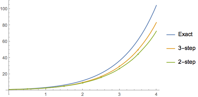
Here is the original numerical example, with 2-step and 3-step solutions:

ClearAll[F];
F[t_, y_] := t + y;
sol2 = Interpolation@abSolve[F, 1., {0., 4., 0.5}, 2];
sol3 = Interpolation@abSolve[F, 1., {0., 4., 0.5}, 3];

sol0 = y /. First@DSolve[{y'[t] == F[t, y[t]], y[0] == 1}, y, t];
Show[
 Plot[{sol0[t]}, {t, 0, 4}, PlotLegends -> {"Exact"}],
 Plot[{Undefined, sol3[t]}, {t, 0, 4}, Mesh -> sol3["Coordinates"], 
  PlotLegends -> {None, "3-step"}],
 Plot[{Undefined, Undefined, sol2[t]}, {t, 0, 4}, 
  Mesh -> sol2["Coordinates"], PlotLegends -> {None, None, "2-step"}]
 ]

The data itself:

abSolve[F, 1., {0., 4., 0.5}, 3]
(*
{{{0.}, 1., 1.},           {{0.5}, 1.5, 2.},          {{1.}, 2.75, 3.75},       {{1.5}, 5.21875, 6.71875},
 {{2.}, 9.57422, 11.5742}, {{2.5}, 16.9683, 19.4683}, {{3.}, 29.3089, 32.3089}, {{3.5}, 49.7041, 53.2041},
 {{4.}, 83.208, 87.208}}
*)

Appendix: Memoization

Note: Memoization. "Memoization" or "cacheing" is a technique to store a computed function value so that on subsequent calls, the value need not be recomputed, only recalled from memory. For function values that are used frequently, this can save considerable time. One has to weigh this savings against greater memory usage. I learned the form mem : f[x_,...] := mem = ... on StackExchange. The mem : ... is a named the pattern and it matches the actual function call.