Introduction
A few weeks ago, I had the privilege of speaking with Michael Foale -- astronaut, astrophysicist, entrepreneur, and Mathematica fan -- about his recent work with the Wolfram Language on the Raspberry Pi. As an experienced pilot, Mike thought he could use the Wolfram Language's machine learning capabilities to alert pilots to abnormal or unsafe flying conditions. Using a collection of sensors attached to a Pi, the Wolfram Language's Classify function would constantly analyze things like altitude, velocity, roll, pitch, and yaw to determine whether the pilot might be about to lose control of the plane. You can read Mike's User story here, his experience with Mathematica on the Space Station Mir here. and the full code for Mike's Imminent Loss Of Control Identification system, or ILOCI, is here.
Getting the Initial Data
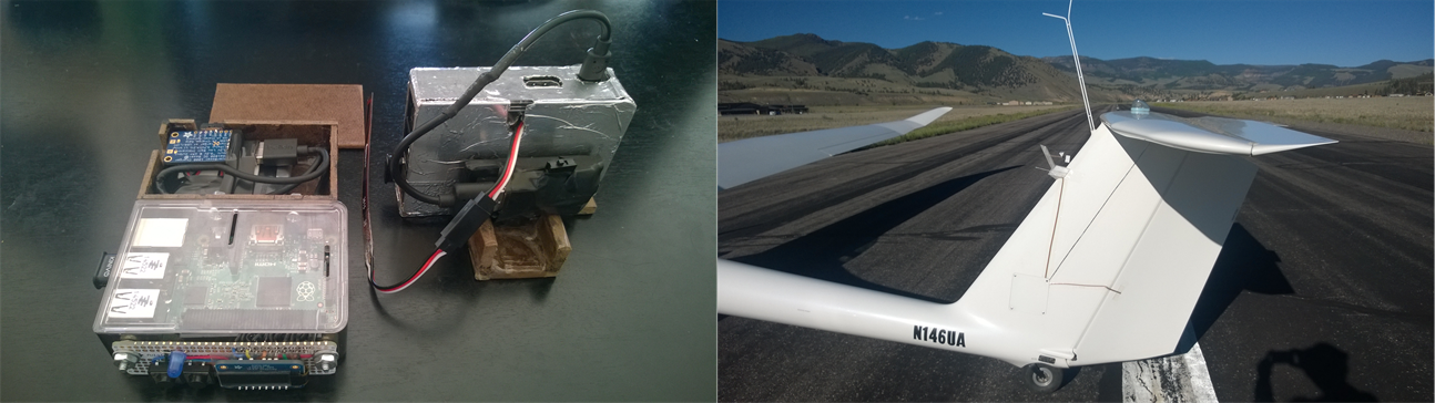
Mike decided that the Raspberry Pi would be a good base for this project because of how easy it is to connect various sensors to the device. In his case, there were 3 sensors he wanted to read from: an accelerometer, an aero sensor attached to the tail, and a flex sensor attached to the rudder. All of these are attached via GPIO pins, which the Wolfram Language can communicate through. In Mike's case, he wrote a MathLink driver in C to do this, but since he began this project we have been pushing to make GPIO communication easier. Now, the Wolfram Language can read from sensors with the DeviceOpen and DeviceRead functions. If Mike were to re-do this project, that would have saved him quite a bit of time and debugging!
Before the Classify function can tell whether current flying conditions are normal or not, it must first learn what normal is. To do this, Mike took his Pi setup on a test-flight where he occasionally forced his plane to stall, or come close to stalling (please, do not try this for yourself!). After landing, he manually separated the sensor readings into "in family" and "out of family" moments -- that is, normal flying conditions and moments where loss of control is imminent.
Importing the Data
For Mike's flights, he had the Pi save data from an initial test flight to a CSV file and had Mathematica import that file to train his Classify function on. For example:
datafile = FileNameJoin[{"","home","pi","Documents","training.dat"}];
data = Import[datafile];
For convenience's sake, I've embedded this same data in a notebook attached to this post, so that you can test and manipulate this data on your own as well. This data, saved under the variable "data", was divided up by Mike into the "in family" and "out of family" periods mentioned earlier:
noloc1 = Take[data, {3500, 3800}];  (* Ground, engine off *)
noloc2 = Take[data, {3900, 4200}]; (* Ground, engine on *)
noloc3 = Take[data, {4500, 4600}]; (* Takeoff, climbing at 60 knots *)
noloc4 = Take[data, {4800, 4900}]; (* Climbing, 70 knots *)
noloc5 = Take[data, {5000, 5200}]; (* Climbing, 50 knots *)
noloc6 = Take[data, {6200, 6300}]; (* Gliding, 42 knots *)
noloc7 = Take[data, {6900, 7100}]; (* Climbing, 60 to 70 knots *)
noloc8 = Take[data, {9200, 9400}]; (* Landing *)
noloc9 = Take[data, {9300, 9400}]; (* Rolling out*)
loc1 = Take[data, {6450, 6458}]; (* Straight stall *)
loc2 = Take[data, {6480, 6484}]; (* Left stall *)
loc3 = Take[data, {6528, 6534}]; (* Right stall *)
loc4 = Take[data, {6693, 6700}]; (* Right Yaw *)
loc5 = Take[data, {6720, 6727}]; (* Left Yaw *)
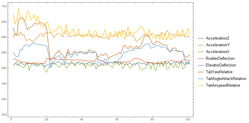
You might notice that the list above doesn't cover the entire dataset. That's because some of the data is kept aside for verification, to ensure the Classify function is recognizing "in family" and "out of family" moments correctly. This is a very important part of training any artificially intelligent program! Below are some plots of the above datasets, just to get a visual feel for what the Pi is "seeing" during a flight.
ListLinePlot[Transpose[noloc4],
 PlotLegends -> {"AccelerationZ", "AccelerationY", "AccelerationX",
   "RudderDeflection", "ElevatorDeflection", "TailYawRelative",
   "TailAngleAttackRelative", "TailAirspeedRelative"}, Frame -> True]
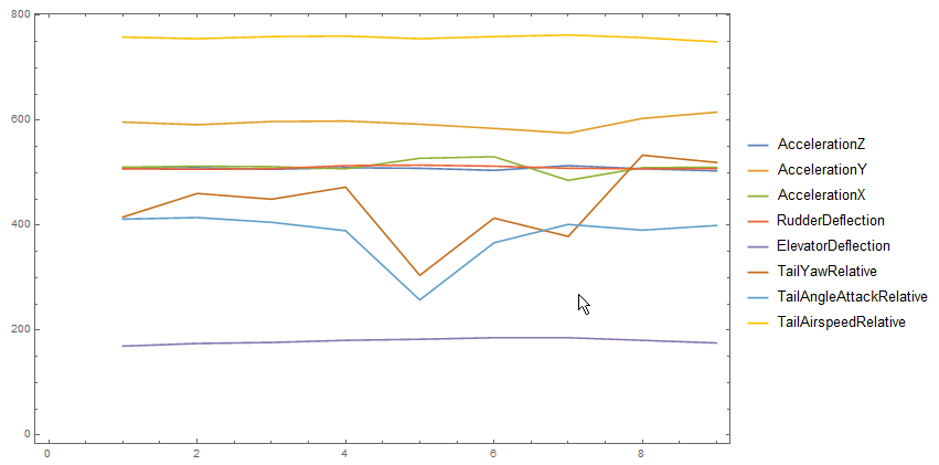
ListLinePlot[Transpose[loc1],
 PlotLegends -> {"AccelerationZ", "AccelerationY", "AccelerationX",
  "RudderDeflection", "ElevatorDeflection", "TailYawRelative",
  "TailAngleAttackRelative", "TailAirspeedRelative"}, Frame -> True]
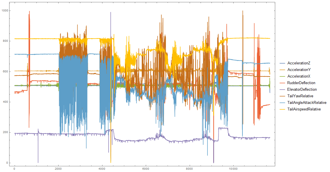
These plots give us a good idea of what happens at some specific instances, but what does the flight as a whole look like? Recall from above that takeoff begins around datapoint 4500, the first stall around 6450, landing around 9200, and the rollout ends around 9400. According to Mike, the rudder movement around 11000 is simply moving the rudder to steer the aircraft back into the hangar.
ListLinePlot[Transpose[data],
 PlotLegends -> {"AccelerationZ", "AccelerationY", "AccelerationX",
  "RudderDeflection", "ElevatorDeflection", "TailYawRelative",
  "TailAngleAttackRelative", "TailAirspeedRelative"}, Frame -> True,
 ImageSize -> Large]
Training the Classifier Data
After separating the data, Mike created Rules to label these moments as "Normal", "Stall Response", "Yaw Response Left", and "Yaw Response Right"; respectively "N", "D", "L", and "R". These Rules teach Classify which patterns belong to which label, so that later on Classify can tell what the appropriate label is for incoming, unlabeled data. Note that the ConstantArray functions simply repeat the data 10 times so the "out of family" moments are not overshadowed by the "in family" ones.
normal = Join[noloc1, noloc2, noloc3, noloc4, noloc5, noloc6, noloc7, noloc8];
normalpairs = Rule[#1, "N"] & /@ normal;

down = Flatten[ConstantArray[Join[loc1, loc2, loc3], 10], 1];
downpairs = Rule[#1, "D"] & /@ down;

left = Flatten[ConstantArray[loc4, 10], 1];
leftpairs = Rule[#1, "L"] & /@ left;

right = Flatten[ConstantArray[loc5, 10], 1];
rightpairs = Rule[#1, "R"] & /@ right;
Finally, with the data segmented and labeled, Mike created a ClassifierFunction able to take live data from the sensors, then quickly tell the pilot when something is wrong and how to correct it.
classify = Classify[Join[normalpairs, downpairs, leftpairs, rightpairs], Method -> {"NeuralNetwork", PerformanceGoal -> "Quality"}]
ClassifierInformation[classify]

Let's use this ClassifierFunction on a couple of the data points that we set aside earlier, to be sure the ClassifierFunction is correct, and to show how a ClassifierFunction is used.
nolocVerify = Take[data, {4600, 4700}];
locVerify = Take[data, {6587, 6595}];

classify[nolocVerify]

classify[locVerify]
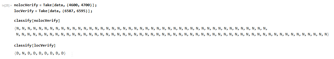
Recall that the ClassifierFunction returns one of 4 labels for each data point: "N" for normal, "L" for left yaw response, "R" for right yaw response, and "D" for down response. Mike's ClassifierFunction perfectly recognizes the first verification set, and comes close to being perfect on the second set. Not bad, given how little data he had to train it with!
This use-case gives a pretty good idea of how the ClassifierFunction works, but for a more in-depth example you can watch this video from Wolfram Research.
Using the ClassifierFunction on Real Data
At the moment I am neither a pilot nor the owner of an airplane, so performing a live test of Mike's ClassifierFunction would be a bit challenging. Fortunately, the Wolfram Language makes it easy to take Mike's recorded data and re-run it as though the ClassifierFunction were receiving this data in real time. First, we need to import the data that Mike recorded in his test flight. We actually did this already, when we called Import on the file containing the data. Next we'll import the timing data from the test flight. This is the absolute time in seconds and microseconds from the beginning and end of the flight, so subtracting the beginning time from the end time gives us the total time of the flight. With the times and the data known, we can determine how often the Pi read in measurements on the test flight. We will use that frame time to "replay" the test flight accurately. Mike's ILOCI system records timing information that we can Import from, but again I'll include it here for the sake of convenience:
timing = {1466861802, 255724, 1466867826, 498879, 11660};
dataseconds = timing[[3]] - timing[[1]];
datausecs = timing[[4]] - timing[[2]];
frametime = (dataseconds + datausecs*1.0*^-6)/(Length[data] - 1)
Now, let's use that frame length to create an animated output of the ClassifierFunction. This goes through the whole dataset and runs at the same rate as the Pi did. If we were actually flying an airplane, this would show us what the Pi thinks about our current environment, whether our motion is "in-family" or "out-of-family".
Animate[
 classify[ data[[frame]] ],
 {frame, 1, Length[data], 1},
 AnimationRate -> (1/frametime),
 FrameLabel -> {{None, None}, {None, "Full Flight Playback"}}
]
This would take a little over 90 minutes to run, and the non-normal readings go by fairly quickly, so let's focus in on some of the more interesting sections. First, let's see the straight stall that was reserved for verification. Again, the ClassifierFunction was not trained using this set -- it is brand new as far as the Classifier is concerned.
Animate[
 classify[ data[[frame]] ],
 {frame, 6580, 6595, 1},
 AnimationRate -> (1/frametime),
 FrameLabel -> {{None, None}, {None, "Stall Playback"}}
]
Notice that the Classifier constantly reads the situation and updates it's classification accordingly. Next let's look at one of the verification sets where everything was normal. It should read as "N" for the entire set:
Animate[
 classify[ data[[frame]] ],
 {frame, 6300, 6400, 1},
 AnimationRate -> (1/frametime),
 FrameLabel -> {{None, None}, {None, "Normal Playback"}}
]
Conclusion
If we go back and count, there is about 60 lines of code. That's all that was needed to create plots, animations, and a neural net-based Classifier that might one day save lives. This is what makes the Wolfram Language such a powerful choice for projects like this -- quick prototyping and a plethora of built-in functions allows users to create some truly unique projects, regardless of experience or expertise. We hope that this will inspire you to start experimenting with your own ideas with the Wolfram Language!


