I'll mention a lesson I experienced.

limited precision (ie on a calculator) can become complicated and need special handling even when arbitrary precision is used. on big problem with it is division.

an example is this: your program must use the result of a previous calculation to decide whether to go left or right on a calendar day / choice. if your precision is "perfect" you know theoretically it will go the right direction. HOWEVER: to divide mathematica must find factors (LCD/GCD etc, eventually), and that is where a flaw can enter

the answer is that some programs must be double careful to proceed in a manner where whether scanning forward or backward through digits never can land on ANY digit at ANY precision which causes their equation to work in one direction but not the other due to "extremely small error". this can be tricky. but your tolerance "at the turning point" cannot be theoretical upon division: you have to develop a way to track which side things will fall on (because ultimately: division is not a perfect thing, not way down deep)

in texas they offer courses on how to do scientific math with limited precision calculators (using non-junk calculators, TI calculators) for just such kinds of "programs" that approach a theory number that can't really be represented. one technique is insuring division isn't used. another is something like newton approx. where tolerance is known ahead and assured.

This seems to be essentially the same what I noted above....... :)

I confess to using bad syntax and descriptive language, but you have essentially answered my questions, which I asked because I am only an intermittent user of the more advanced features...advanced to me...in Mathematica.

The application is an esoteric one of applying Einstein's radiation pressure model to a variety of scenarios. In the 1905 paper by Einstein, he describes how the Poynting Vector is impacted by detection in a moving frame...it is just a radar problem: what is the actual frequency that impacts a moving object? From Einstein's perspective, the radiation is Doppler shifted into the moving frame and then the interaction occurs.

I converted this model into a linear model using photons and flux and, ultimately, radiation pressure. Einstein's model omits what I have called a compression factor. This is just a geometrical factor that allows the number of photons that impact an object to depend on whether the object is moving toward a source or against the source of radiation. An example is that of a helium filled balloon held in a wind. When the balloon is stationary, the number of molecules of air hitting the balloon is constant. When I let the balloon go, it quickly accelerated to the wind speed and the number of wind molecules hitting the balloon drops nearly to zero. Likewise, if I walk into the wind holding the balloon, more molecules hit the balloon per unit time increasing the force on the balloon.

I generalized these factors for movement of an object obliquely through a radiation flux, but for many scenarios, we are moving directly into or against the radiation. I then began a parametric study of the effective radiation pressure on various sized objects moving at various speed in various directions. The question I posed was how to solve one of these scenarios, which is somewhat of a science fiction type, though I have also looked at solar sails, radiation sails in general, radiation forces on spacecraft, and particle accelerators. Some of the results are quite surprising and too quickly dismissed as having no practical consequence.

Thanks you for your patience and forbearance.

Luther.

Welcome to Wolfram Community! Please make sure you know the rules: https://wolfr.am/READ-1ST

Please post your full code of what you are trying to do.

Please make sure you know read all rules: https://wolfr.am/READ-1ST

The rules explain how to format your code properly. If you do not format code, it may become corrupted and useless to other members. Please EDIT your posts and make sure code blocks start on a new paragraph and look framed and colored like this.

int = Integrate[1/(x^3 - 1), x];
Map[Framed, int, Infinity]

Have you tried taking a limit as b approaches 1 from the left side?

I'm not sure what is confusing about .99 being less than .999, or what that might have to do with taking a limit (which is what I had asked). I will add that the entire thread has been remarkably murky in terms of stating what exactly is wanted and what exactly has been tried. Let me comment on some related issues that I believe are being raised.

(1) Precision in a plot range. The input shown in an earlier post does not produce a plot (this fact, and the error message, should have been noted in that post).

ff = ((1 + b)^2)/Sqrt[1 - b^2]
LogLogPlot[ff, {b, .9999999999999999999, .99999999999999999999}]

(* During evaluation of In[122]:= Plot::plld: Endpoints for b in {b,0.9999999999999999999,0.99999999999999999999} must have distinct machine-precision numerical values.

Out[122]= LogLogPlot[ff, {b, 0.9999999999999999999, 
  0.99999999999999999999}] *)

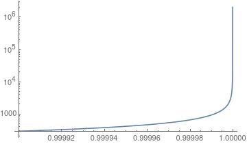
What to do about it? One remedy is to widen the range. You can let the right bound be 1 for example. This next will give a picture that might be informative.

LogLogPlot[ff, {b, .9999, 1}, PlotRange -> All]

(2) Solving runs into precision problems. This can be alleviated by explicitly using higher precision in the input. Notice the back-tic in the input below. It parses the input number to 20 digits precision.

Solve[ff - .99999999999999`20 == 0, b]

(* Out[111]= {{b -> -5.00000000000006875*10^-15}} *)

(3) More confusion. If the interest is in b approaching 1, that's not the same thing as ff being close to 1. So the use of Solve seems unhelpful for the stated problem (as best I can interpret it). I would guess what is wanted is for ff to be large and then find b. This requires considerable precision, roughly twice as many digits in for the number you want out. Some analysis of the expression might help to explain this (e.g. expand in Puisiux series centered at b=1). Anyway, here is an example. Notice the decimal point is at the right rather than left side of the value for ff.

NSolve[ff - 99999999999999999999.`40 == 0, b]

(* Out[139]= {{b -> 0.9999999999999999999999999999999999999992}} *)

What do you mean by "solve"? Are you looking for the limiting value? Fi so, it blows up (that is, goes to plus or minus infinity depending on the direction of approach).

I understand you have a function f given by the following equation e1

In[1]:= e1 = f == (1 + b)^2/Sqrt[1 - b^2]

Out[1]= f == (1 + b)^2/Sqrt[1 - b^2]

I square both sides and obtain

e2 = #^2 & /@ e1

f^2 == (1 + b)^4/(1 - b^2)

Having in mind that ( 1 - b^2 ) = ( 1 - b ) ( 1 + b ) you may guess that you will arrive at an equation with b^3. FullSimplify does the job

In[3]:= e3 = e2 // FullSimplify

Out[3]= (1 + b)^3/(-1 + b) + f^2 == 0

Now use

e4 = Solve[e3, b]

and you will get three equations for b (two with imaginary parts) which give you b when you plug in f. With Mathematica's numerical power this should give you an answer to your question.

For example

Block[{$MaxExtraPrecision = 500}, N[e4[[1]] /. f -> 10^80, 6000]]