We present simple and workable solution for construction of multivariate Brownian Bridge Process that can be used for analysis of multivariate patterns in conditioned distribution based on Wiener process. The ability to derive adjacent distributions based on BB process leads to interesting applications in Finance where we examine options on maximum of n-assets subject to upper barrier boundary. The use of Ito Process as a wrapper simplifies the construction argument and leads to elegant solution of the task.
Introduction
Let' s recall that BB denoted as $(H (t))$ is continuous - time adapted version of the Brownian motion and it differs from the latter in one aspect - its probability distribution is conditional probability of a Wiener process $(W (t))$ with condition $H_0 =H_T = \alpha$
The linkage of Brownian Bridge to the standard Brownian motion (W (t)) from [0,0]] on [0, T] can be seen from the following definition $X (t) = W (t) - t/T W (T)$. The second expression is a function of time [ScriptT] from values [0, 0] on [T, W (T)]. By subtracting t/TW(T) from the Brownian motion W (t), we ensure the condition of X (t) = X (T) = 0.
Properties of the BB process
On the defined line [0,T] the random variables  are jointly normal since their random components $W(t1), W(t2)...W(tn)$ are normal. Therefore, the BB process from [0 to 0] on the time line $[0,T]$ is a Gaussian process with mean = 0
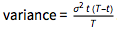
Additional proof of normality of BB process can be seen from the probability density of this process:
Clear[bbp, s, T, t, a, b];
bbp = BrownianBridgeProcess[\[Sigma], {s, a}, {T, b}];
PDF[bbp[t] /. {s -> 0, a -> 0, b -> 0}, u] // Simplify
Plot[% /. {\[Sigma] -> 0.03, T -> 1, t -> 0.5}, {u, -0.05, 0.05},
 PlotTheme -> "Business",
 PlotLabel -> Style["PDF of the BB Process", Purple, 15]]
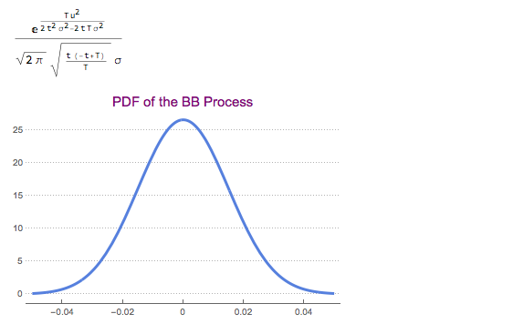
Relaxation of assumptions on the parameters values leads to generic BB process evolving along the time line [0, T] and taking values [a, b], both non - zero. This BB process then becomes $X(t)+a+t(b-a)/T$ for $0<=t<=T$ where  , the BB process from [0 to 0[ defined above. Since we have added a non-random function to the Gaussian process, we obtain again a Gaussian process, now with a different - 'shifted' mean $= a+t(b-a)/T$, but the same variance = $(\sigma^2 t (T-t))/T$
Relation of BB to Ito process
We cannot express the BB process in terms of Ito stochastic integral with deterministic integrand since the BB process has non-monotonic variance. From the variance expression above it is clear that the variance increases on the interval 0<=t<=T/2 and decreases on T/2<=t<=T.
Plot[(\[Sigma]^2 t (T - t))/T /. {T -> 1, \[Sigma] -> 0.05}, {t, 0,
  1}, PlotLabel -> "Variance of the BB process"]
However, we can define a process with the same distributional properties as the IBB process from [0 to 0] that is known as 'scaled stochastic integral'. Let's define 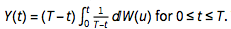 . Then the integral
 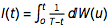 is essentially a Gaussian process provided t<T and he random variables $Y(t1)=(T-t1) I(t1), Y(t2)=(T-t2) I(t2)$.... are jointly normal and therefore expressible through Ito process. This can be directly confirmed in Mathematica by providing Ito Process wrapper for the Brownian Bridge Process.
ItoProcess[bbp] // TraditionalForm
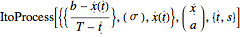
This shows that the BB process is an Ito Process with $drift = (b-x(t))/(T-t)$ and volatility parameter $= \sigma$
Multi-variate BB process
The ability to define the BB process as a special form of Ito process offers a number of advantages. One of particular interest is the construction of multi-variate Ito processes that are well--defined and easily applicable in Mathematica. This means that the construction of multi-variate BB process is feasible through Ito Process definition.
BB process in Finance
BB process in unique in its definition and specification. The fact it is a derived version of the Brownian motion with time-dependent path offers a number of advantages. It allows to model intermediate paths when the initial and terminal points are fixed.This is useful to model yields on assets with 'pull-to-par' feature.
BB process found its way into finance on two other counts:
We focus on the first case and demonstrate how multi-variate BB process can be used to value multi-factor option with upper barrier ceiling. For this, we define:
10 variables = can be returns on financial assets
Initial yields are in the range of 1% - 5%
We set the condition: Initial yields = final yields: a=b
We defined random covariance matrix
Evaluation process starts at t=0 and ends at T=1 (year)
We will model the multi-variate BB process and the multi-variate Ito Process with BB-adjusted drift (bbdrift) and random covariance matrix (cov)
m = 10;
iv = RandomReal[{0.01, 0.05}, m];
CM[n_, min_, max_] := #.Transpose[#] &@
   RandomReal[{min, max}, {n, n}];
cov = CM[m, -0.01, 0.02];
We define variables for the process:
    vars = Table[Symbol["x" <> ToString[i]], {i, m}];
    xtvar = Table[vars[[i]][t], {i, m}];
    tf = Table[Symbol["b" <> ToString[i]], {i, m}];
    lab = Table["BB Plot No " <> ToString[i], {i, m}];
and define the drift function:
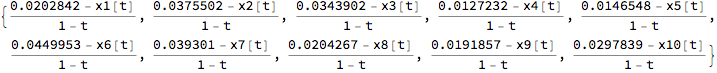
bbdrift = (tf - xtvar)/(T - t)

We replace the variables with actual values:
tf = iv;
bbdrift = (tf - xtvar)/(T - t) /. T -> 1
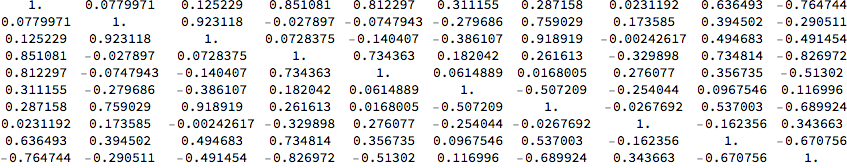
Here we specify the BB process as the Ito Process with vector-valued input and the correlation matrix:
Grid[cov // Correlation, ItemSize -> Small]
ip2 = ItoProcess[{bbdrift, IdentityMatrix[m]}, {vars, iv}, t, cov];
ProcessParameterQ[ip2]
True
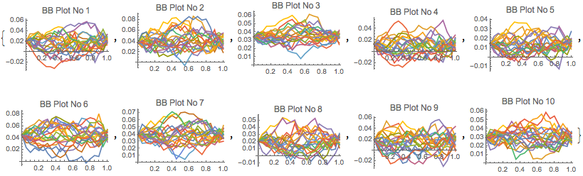
We run the simulation of 5,000 paths per asset and visualise some sample paths
SeedRandom[Method -> "MersenneTwister"] ;
path2 = RandomFunction[ip2, {0, 1, 0.05}, 5000,
  Method -> "StochasticRungeKutta"];
Evaluate@Table[
   ListLinePlot[path2["PathComponent", i]["Path", Range[20]],
    PlotRange -> All, PlotLabel -> lab[[i]], ImageSize -> 150], {i,
    m}] // Quiet
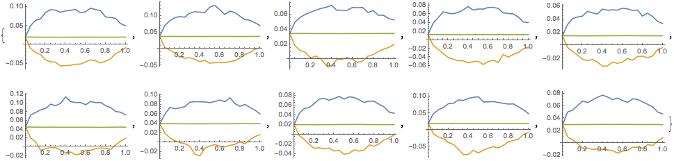
Range statistics for each asset
Based on the simulation run, we define the Max, Min and Mean values per each asset yield
Table[ListLinePlot[{TimeSeriesThread[Max, path2["PathComponent", i]],
   TimeSeriesThread[Min, path2["PathComponent", i]],
   TimeSeriesThread[Mean, path2["PathComponent", i]]}], {i, 1, m}]
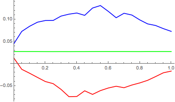
Max, Min and Mean for the entire family of all assets
and then create the 'global' measures - Max, Min and Mean values across all 10 assets:
pmax1 = TimeSeriesThread[Max, path2];
pmn0 = TimeSeriesMap[Mean, path2];
pmn1 = TimeSeriesThread[Mean, pmn0];
pmin1 = TimeSeriesThread[Min, path2];
ListLinePlot[{pmax1, pmn1, pmin1}, PlotStyle -> {Blue, Green, Red}]
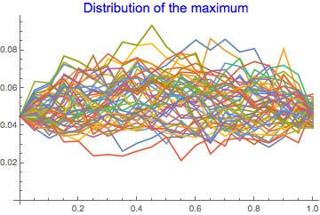
Distribution of the Max
We are interested in the maximum value per each path along the time line. We therefore create the 'distribution of the maximum '
maxD = TimeSeriesMap[Max, path2];
ListLinePlot[maxD["Path", Range[50]],
 PlotLabel -> Style["Distribution of the maximum", Blue, 15]]
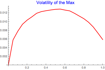
The volatility of the maximum follows general pattern of increasing volatility on the interval 0<=t<=T/2 and decreasing on the remaining part.
TimeSeriesThread[StandardDeviation, maxD];
ListLinePlot[%, PlotLabel -> Style["Volatility of the Max", Blue, 15],
 PlotStyle -> {Red, Thick}]
We also examine the distribution of the Maximum
SmoothHistogram[maxD, Filling -> Axis, FillingStyle -> Opacity[0.25, Pink],
 PlotTheme -> "Business"]
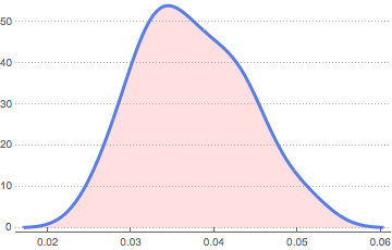
The distribution is clearly non-normal
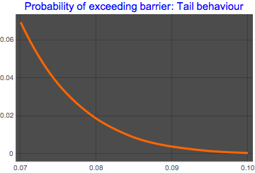
Using the Max distribution above, we now build a smooth kernel distribution that we us further in other calculations. In particular, we way want to examine the tail behaviour as a function of upper barrier. For this purpose, we look at the probability of max value exceeding barrier for the entire family of components:
maxDD = SmoothKernelDistribution[maxD];
Plot[Probability[x > u, x \[Distributed] maxDD], {u, 0.07, 0.1},
 PlotTheme -> "Marketing",
 PlotLabel ->
  Style["Probability of exceeding barrier: Tail behaviour", Blue, 15]]
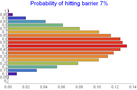
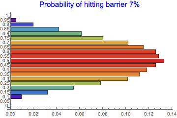
We can equally pose a different problem and look at the 'slice distribution' and examine the probability of hitting barrier as we move in time. This is presented in the chart below where we look at the probability of hitting barrier of 7%
Table[Probability[x > 0.07, x \[Distributed] maxD[i]], {i, 0, 1,
   0.05}];
BarChart[%, BarOrigin -> Left,
 PlotLabel -> Style["Probability of hitting barrier 7%", Blue, 15],
 ColorFunction -> Function[{height}, ColorData["Rainbow"][height]],
 ChartLabels -> Table[i, {i, 0, 1, 0.05}]]
Multi-factor option with multivariate BB process
Knowing the distribution of multivariate BB process with max values allows us defining various problems on this quantity. Of of them is option valuation on the max on n-assets subject to barrier restrictions. Availability of max distribution simplifies the task in many ways - the option can be built as conditional expectation. We demonstrate he concept on the global distribution family:
Plot3D[Expectation[x - k \[Conditioned] k <= x <= h,
  x \[Distributed] maxDD], {k, 0.06, 0.08}, {h, 0.08, 0.1},
 ColorFunction -> "DarkRainbow", PlotLegends -> Automatic,
 AxesLabel -> {"Strike", "Barrier"},
 PlotLabel ->
  Style["Barrier-bounded option on the max of 10 assets", Blue, 15]]
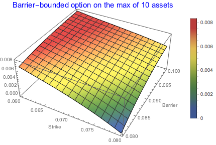
For the call option we observe:
Option value per period
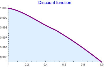
In practice, we are more interested in option valuation on 'slice distribution' when the BB process moves in time. To accomplish this task, we first build the discount function
dfint = Interpolation[{{1/12, 0.0025}, {3/12, 0.0038}, {1/2, 0.0044}, {1,
     0.0055}}, InterpolationOrder -> 2];
DF[t_] := Exp[-dfint[t ] t] // Quiet
Plot[DF[x], {x, 0, 1}, PlotLabel -> Style["Discount function", Blue, 15],
 PlotStyle -> {Thickness[0.01], Purple}, Filling -> Axis,
 FillingStyle -> LightBlue]
We value these call options as discounted conditional expectation of max value exceeding the strike and staying below the upper barrier. Call option values for strike k=7% and barrier h=10% are shown below:
Table[{i,
   DF[i] Expectation[
     x - k \[Conditioned] k <= x <= h /. {k -> 0.07, h -> 0.1},
     x \[Distributed] maxD[i]]}, {i, 0, 1, 0.05}];
ListLinePlot[%,
 PlotLabel ->
  Style["Option value per period: k=7% and h=10%", Blue, 14],
 Filling -> Axis, FillingStyle -> LightGray,
 PlotStyle -> {Magenta, Thickness[0.01]}]
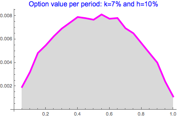
We observe the following:
For BB process with fixed initial and final values (a=b), the maximum value occurs at T/2. This consequence of peal variance at this point
Option valuation resembles variance patterns and follows typical convex profile
The optimal timing occurs at the maximum point of the graph above
Conclusion
Multivariate BB process in Mathematica can be easily built using its relationship to the Ito Process. This opens multiple avenues for the process analysis and provides useful basis for building of auxiliary processes used in finance. Distribution of max or min based on multivariate BB processes is one the examples presented in this note.
The analysis of BB process and its applications can be extended further. Different stating and final values, variance relaxation over time and addition of heavier tails can be explored in further research.
 Attachments:


