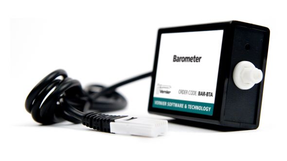
With all the hurricanes raging in the Atlantic, I got curious about doing some home-grown science by tracking barometric pressure in my home state of Illinois. I decided to use Vernier's Barometer sensor, because it has built-in Device Framework support.

Tracking barometric pressure requires patience, because it takes several days before you have enough data that is interesting enough to look at: Taking measurements for just one minute won't cut it (unless you want to stare at a plot with a very flat line in it). You also need a reliable system for collecting and storing data. Something that can survive a computer reboot or a temporary power outage.

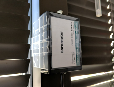
Here is the barometer in a more operational setting:

To build this reliable system, I used the Windows task scheduler (on Mac and Linux something like cron will serve the same purpose). The details of the scheduled task creation are a little too technical for this post, but the code is located here. After creating the scheduled task, it will run every 5 minutes (as long as the computer is powered on):

C:\Users\arnoudb> schtasks
[...]
Folder: \Wolfram
TaskName                                 Next Run Time          Status
======================================== ====================== ===============
Vernier Barometer Experiment             9/25/2017 1:26:00 PM   Ready
[...]

The key part of the scheduled task is the following bit of WL code. It simply connects me to the cloud (using my wolfram id and password), opens the sensor device, takes one pressure reading and stores it in the DataDrop cloud:

$CloudBase = "https://www.wolframcloud.com";
CloudConnect["arnoudb@wolfram.com",password];
barometer = DeviceOpen["Vernier"];
pressure = DeviceRead[barometer];
bin = Databin["ovjo5DbK"];
DatabinAdd[bin, <| "pressure" -> pressure |> ];

I store my password (encrypted) as a LocalSymbol["password"] and then set InitializationValue[$Initialization] to decrypt it automatically for each new kernel session.

This Databin is publicly readable at this URL so anyone can use the data from it:

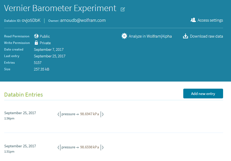
At this point, it is time to let the computer do its thing for a week or so and let the data accumulate. Very little human interaction is required, except perhaps for making sure data is being added. Then, after a couple of weeks, it is time to take a look at the collected data and analyze it. First we fire up a notebook and get the databin:

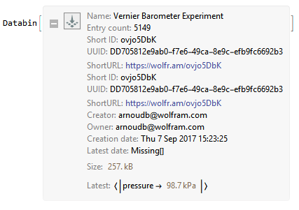
bin = Databin["ovjo5DbK"]

The output is a Databin expression, with all the meta-data defined:

To get the actual data, you can request the TimeSeries of the data:

ts = TimeSeries[bin]

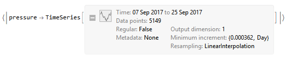
Unfortunately, 7 out of the 5149 measurements failed (0.136%), so a little data scrubbing is needed to remove those:

ts2 = TimeSeries[Cases[Normal[ts["pressure"]], {_DateObject, Quantity[_, "Kilopascals"]}]]

Now the cleaner version of the TimeSeries can be plotted:

DateListPlot[ts2, Filling -> Axis, 
 FrameLabel -> {"Date", "Pressure (kPa)"}, 
 PlotLabel -> "Pressure in Illinois"]

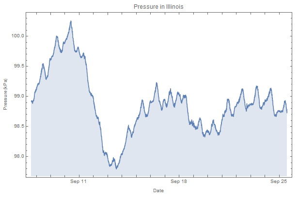
The biggest dip in the plot corresponds to the moment when the post-tropical low pressure system of Irma reached Illinois.

If you want to take a closer look at this code, you can find the notebook here on GitHub.