This posting is motivated by an earlier posting: Plotting a specific branch of a multi-valued complex function. However it uses an entirely different method to representi the function, showing the entire function and not just a single branch.
The function is:
f[z_] := Sqrt[z (z - 1)]
This is a two-valued function with the values given by:
wvalues = w /. Solve[f[z]^2 == w^2, w]
giving:
{-Sqrt[-1 + z] Sqrt[z], Sqrt[-1 + z] Sqrt[z]}
The following is a dynamic (in a notebook) display of the function on a Riemann surface:
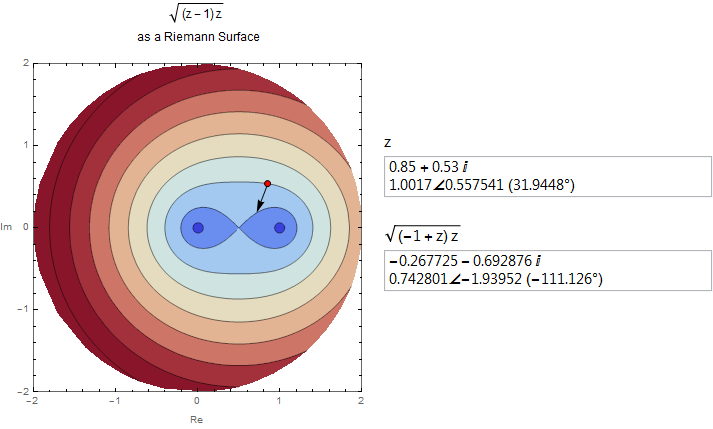
The background is just the modulus of the function and is included to help orient us on the function. The red point is a locator that indicates the position on the Riemann surface. A vector is attached to the locator that gives the value of the function at that location. The dark blue spots are the function zeros at z = 0 and 1. On the Riemann surface the function is single-valued and continuous. The function can be explored by dragging the locator. There will be no discontinuities or jumps in the black vector representing the value.
If the locator is dragged around both of the zeros it will return to its initial value with one circuit. If it is pointing inward it will always point inward. If it is pointing outward it will always point outward. If the locator is dragged around only one of the zeros it will require two circuits to return to its original value. One circuit will reverse the sign of the function and of course the inward-outward pointing. We really are moving on a Riemann surface for this function.
This type of display is a feature of my Presentations application. It uses a routine, CalculateMultivalues, useful when calculating the values of a multifunction while tracing out a path in the complex plane. In this case it will often be convenient to have each root of the multifunction follow a continuous path. If we trace the function in small enough steps then it will generally be possible to identify the new set of roots with the previous set of roots by a permutation. This can be done by calculating the distances between all pairs of roots, and then considering it as an 'assignment problem' that can be solved by the Mathematica LinearProgramming routine to minimize the total distance between the new set and the previous set.(Otherwise the root values returned by Mathematica will undergo jumps so that a particular single root value will be discontinuous.)
Complex functions are often better explored with multiple displays. Here is a display representing the function as modulus and argument surfaces.
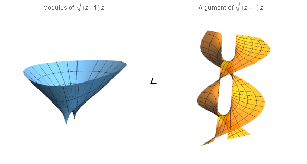
There are two main branches on the argument surface that sweep from - Pi to Pi, but there are connections between them near the zeros. The argument surface has one artifact in that the top edge should be glued to the bottom edge. The surface should probably be stretched vertically and then wrapped into a circle matching the two edges. The angular position on the circle would be the argument value. It might be a nice surface to print 3D.


