This post was originally published at Ultimaker.
Pioneer Chris Hanusa led a Mathematica and 3D printing workshop where he shared resources to help attendees get up and running with the program and 3D printing. At the end of the information-rich workshop, attendees learned how to to use Mathematica to create several 3D printable objects, including name tags.
In October, at my invitation, Assistant Professor Chris Hanusa of the Math Department at Queens College led an Introduction to 3D printing with Mathematica workshop for educators at NYUs ITP in New York City. Chris is a mathematician and a designer who creates beautiful objects inspired by math (you can see his work on his website hanusadesign). Chris creates his objects and shares the math behind them on his site. He has also written several tutorials on his blog mathzorro.com about how to use Mathematica to create 3D objects. There is a great deal to learn about Mathematica before one can start designing printable 3D objects, and during the workshop Chris worked to provide the attendees with enough information to be just a little bit dangerous. Without a question, Mathematica is the kind of application that one needs to see in action, and then spend quite a bit of time with processing the information and doing further exploration on ones own.
Chriss teaching style encourages independence. He shows his college students how to rely on Mathematicas extensive documentation, and he provides well-scaffolded tutorials to follow so that his students develop their understanding and confidence.
Mathematica is not a CAD package, nor was it created with 3D printing in mind. However, one can use Mathematicas programing language to create printable 3D objects, basically watertight, mesh files and export them as STLs or OBJs. Like other programming languages (Processing, Openscad, OpenGL) that can create 3D objects with code, you dont have the ability to drag and drop shapes. Basically, you create statements that generate nodes or vertices in 3D space. By specifying coordinates, you can then apply rotate, scale and translate transformations. You can use parametric curves, vector functions, and trigonometry to create your geometric objects. Remember when you asked in Trig class "When will ever use this?" Well, youll use your trig in Mathematica to create 3D printable objects. Math class would have been very different for me if I had access to both Mathematica and 3D printing back when I was in high school.
What I like about Mathematica (and Processing and OpenSCAD) is the algorithmic approach to generating objects. While Processing uses a sketch metaphor and OpenSCAD employs an editing window, Mathematica uses notebooks. For each of these options, programmers start with a general idea of a task for their computers to perform. Programmers then flesh out their general ideas into complete, unambiguous, step-by-step procedures to carry out their tasks. Such procedures are called algorithms. An algorithm is not the same thing as a program. A program is written in some particular programming language, like C, Java, Python, or the Wolfram Language. An algorithm is more like the idea behind the program. An algorithm can be expressed in any language, including English.
When you know what you want your program to do, many programmers find it helpful to write a description of the task or tasks. That description can then be used as an outline for their algorithm. As a programmer refines and elaborates on their description, gradually adding more details, they eventually end up with a complete algorithm that can be translated directly into a programming language. This method is called stepwise refinement, and it is a type of top-down design. As you proceed through the stages of stepwise refinement, you write out descriptions of your algorithm in pseudo-code, the informal instructions that imitate the structure of your program without complete details or the perfect syntax of actual code. Pseudo-code is where you figure out what kinds of data your program needs and what kind of data it returns. This is also the step where you think about the best way to solve the problems that you're going to run into during the project, and to you get to figure out solutions to try before even starting to write code.
Think of programming as a process of logical problem-solving. Your two big challenges are a) learning the syntax, and b) applying your logical problem-solving skills to an unfamiliar domain. When I taught programming at Saint Anns School in Brooklyn, NY, I told my students who were learning a new language to break things down into four areas:
- Code-readingbe able to look at code and figure out what its doing. Code-reading means two things:
Being able to understand what a particular line of code is doing - understanding the syntax of the program.
It also means understanding something called the control flow of the program: when the program executes a line of code, what will it execute next?
- Pseudo-codeThis is where you do a lot of thinking and not a lot of writing code. Because most projects start with a vague idea, or an English description, this step helps turn your project into something that is approachable as a program. It forces you to define and explain what you're trying to do very precisely.
- Code-writingIt can be intimidating to try and figure out how to express what you're trying to do with an unfamiliar syntax of a programming language. However, if you've done a good job with the pseudo-code, writing your code should be in some ways the simplest step. Youre performing a translation from the precise and clear concepts you've figured out to the syntax of the programming language in question. As you write the code, you'll figure out some issues that your original design or pseudo-code didn't address. You'll improvise, double back, and sometimes change your entire design. But the more you separate the simple writing of code from the hard work of figuring out what you want the code to do, the happier you will be in the long run.
- DebuggingThis is the process of testing and fixing the problems in a program that you've already written. Unfortunately, this is the step that will generally take most of your time. While occasionally you will be able to write a program that's bug-free, generally your program will either not work immediately or it will do something completely unexpected. Learning techniques for figuring out what's wrong (and even more important, solving the problem) is important. The more code you write and the longer your programs become, the harder problems become to track down and deal with.
Start small, modify, test and build incrementally. When you work in Mathematica, instead of modifying code that works, make a copy and modify the copy. This way youll have a record of what you started with that you can always return to at a later date.
Mathematica is also capable of nested commands. But ease into this. Until you know how each command works (what information a command takes and what it returns) you may want to consider separating the commands out. As you become more experienced, nest away with confidence.
During the workshop, Chris pointed out a few things that were helpful to keep in mind:
- Mathematica is case sensitive.
- All built-in Mathematica functions are spelled, capitalized, and follow CamelCase rules.
- It is important to distinguish between parentheses (), brackets [], and braces {}: Parentheses (): Used to group mathematical expressions, such as (3+4)/(5+7). Brackets []: Used when calling functions, such as N[Pi]. Braces {}: Used when making lists, such as {i,1,20}.
- To calculate an expression, use Shift-Return.
- To find the options of a given function, highlight it in the notebook and then press Command+Shift+F.
- A semicolon can be used to suppress output.
- Mathematica has four types of equals: =, ==, :=, and ===.
- Assignment: To define a variable to store it in memory, use =. For example, to define z to be 3, write z=3.
- Test for equality: Use == to check for equality. For example, 1-1==0 will evaluate to True and 1==0 will evaluate to False.
- Set Delay: Use := when you want to evaluate the function when it is called rather than when it is assigned . (This is advanced.)
- SameQ: Use === to test whether two expressions are identically the same.
Adding comments to your notebook will help you remember what your intentions were when you look back on your notebook months later. Comments are also invaluable for other people who are navigating through your notebook. To write a sentence, create a new text cell by clicking below a cell. When the cursor turns horizontal type Option-7, or right click and navigate to Insert New Cell > Text.
Use the documentation. If you are having trouble with a certain function, use the ? command to ask for help. For example enter ? Table and the output will be a yellow box with a quick synopsis of the command. For more detailed information, click the blue >> at the bottom right of this yellow box. This will open the Documentation Center which gives examples of using the command in action, available options for this command, and anything else you might want to know about the command.
The following three statements represent a sphere, a cuboid and a cone:
Sphere[{0, 0, 0}, .28]
Cuboid[{-.05, -.05, .26}, {.05, .05, .35}]
Cone[{{0, 0, 0}, {0, 0, -1}}, .3]
You can also combine them using a list
Graphics3D[{
Sphere[{0, 0, 0}, .28],
  Cuboid[{-.05, -.05, .26}, {.05, .05, .35}],
  Cone[{{0, 0, 0}, {0, 0, -1}}, .3]
  }]
They are combined, but if you press Shift Return, I suspect you may not get what you expect.
In order to see all the objects combined you have to pass these objects from Graphics3D[] to Show[]:
sphere = Graphics3D[Sphere[{0, 0, 0}, .28]]
cuboid = Graphics3D[Cuboid[{-.05, -.05, .26}, {.05, .05, .35}]]
cone = Graphics3D[Cone[{{0, 0, 0}, {0, 0, -1}}, .3]]

Show[sphere, cuboid, cone]
Like other programming languages, there's often more than one way to do do the same thing:
shapes = {
Sphere[{0, 0, 0}, .28],
Cuboid[{-.05, -.05, .26}, {.05, .05, .35}],
Cone[{{0, 0, 0}, {0, 0, -1}}, .3]}
Map[Graphics3D, shapes]
Show[Map[Graphics3D, shapes]]

Graphics3D[Table[Sphere[{i, 0, 0}, .2], {i, 0, 10}]]
To get the workshop attendees started, Chris created a Mathematica Basics Crash Course and a 3D Graphics in Mathematica notebook.
If you're new to Mathematica, open Chriss notebooks and execute each command by placing your cursor at the end of the line and pressing Shift+RETURN. Not everything will make sense right away, and thats okay. Mathematica is packed with information and functionality. At the beginning just try to appreciate what it is doing, and then marvel at what might be possible when you have more experience.
Mathematica has a large number (195) of built-in polyhedra that you can create, export and print. They are accessible using the command PolyhedronData[]. How do I know how many polyhedra Mathematica can represent? Execute the following statement:
Length[PolyhedronData[All]]
To find out the properties associated with PolyheronData[] execute the following command:
PolyhedronData["Properties"]
And here is a handy statement to explore all the polyhedra:
Manipulate[
Column[{PolyhedronData[g], PolyhedronData[g, p]}], {g,
 PolyhedronData[All]}, {p,
 Complement @@ PolyhedronData /@ {"Properties", "Classes"}}]
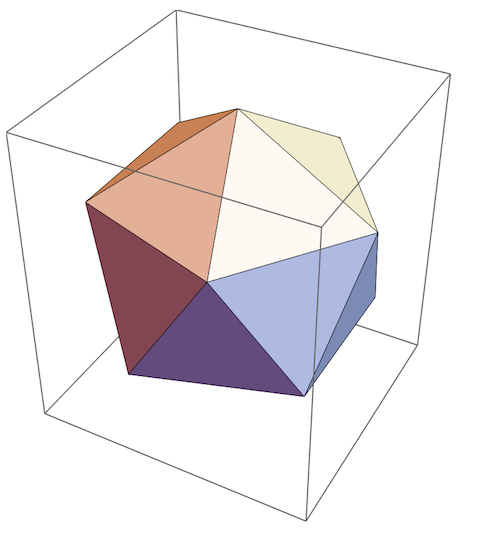
Here how to create a 3D object that you can see and then export:
myShape = Graphics3D[PolyhedronData["Icosahedron", "Faces"]]
Save your notebook. Then to export the object as an STL file :
Export[NotebookDirectory[] <> "myFile.stl", myShape]
And then to see the STL:
Import[NotebookDirectory[] <> "myFile.stl"]
Back to name tags
Name tags or nameplates often seem to me to be the Hello World of 3D printing. They are generally pretty simple to create with a CAD package and they provide an easy introduction to 3D space. There is nothing inherently wrong with creating name tags or nameplates, but I think 3D printing is capable of so much more, and I try to advocate for finding the real potential for 3D printing in education. Yet here I am, encouraging you to use Mathematica to create a name tag. Why? Because I think it is helpful to start off with a familiar object in an unfamiliar context. Remember, Mathematica wont let you click and drag. You are going to have to build a name tag from the ground up, and in the process, youre going to become familiar with some of Mathematicas mesh commands.
At its simplest, to make a name tag, youre going to need a base and then a top. Remember that an STL file is a watertight mesh. That means that where the base and the top meet you will need to eliminate the top surface on the base and the bottom surface of the top. Lets start with some text:
Text[Style["Ultimaker", Bold, FontFamily -> "Futura", FontSize -> 50]]

You now need to convert this text to a 2D mesh. To do that you use the command DiscretizeGraphics[]:
meshText2d = DiscretizeGraphics[
 Text[Style["Ultimaker", Bold, FontFamily -> "Futura",
   FontSize -> 50]], _Text]

To make the 2D mesh 3D use RegionProduct[] with the mesh and a vertical line:
RegionProduct[meshText2d, Line[{{0.}, {5.}}]]

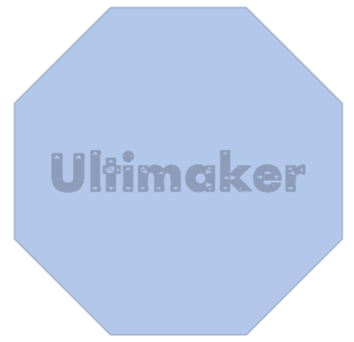
Next youll create a 2D mesh of a polygon to act as the base:
base = DiscretizeGraphics[Graphics[{RegularPolygon[8]}]]

To see the two meshes together:
Show[{RegionResize[base, 1.3], RegionResize[meshText2d, 1]}]
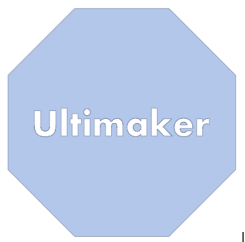
Next you need to remove the surfaces where the two meshes intersect (RegionDifference[]) and make the base big enough to support the text (RegionResize[]):
polygon = RegionResize[base, 1.3];
text = RegionResize[meshText2d, 1];
intersection = RegionDifference[polygon, text]
Now you need to create boundaries from the two regions so that you can create walls:
bdrypolygon = RegionBoundary[polygon]
bdrytext = RegionBoundary[text]


Now you need to build the actual mesh. Youll need to create 3 levels: the floor, the top of the base and the top of the text (You must use a floating point number):
level0 = 0.;
level1 = 0.1;
level2 = 0.15;
Now its time to put all the parts together:
Show[{
 RegionProduct[polygon, Point[{{level0}}]],
 RegionProduct[bdrypolygon, Line[{{level0}, {level1}}]],
 RegionProduct[intersection, Point[{{level1}}]],
 RegionProduct[bdrytext, Line[{{level1}, {level2}}]],
 RegionProduct[text, Point[{{level2}}]]
 }]
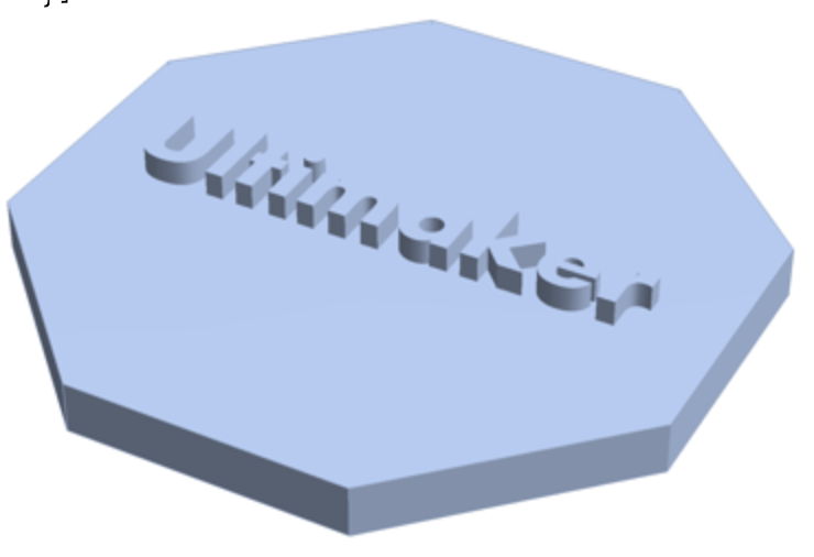
Export and Import. You can use the % as shorthand for the last thing you created:
Export[NotebookDirectory[] <> "nametag.stl", %]
Import[NotebookDirectory[] <> "nametag.stl"]

If the export doesnt work, it could be that your notebook hasnt been saved yet. Save the notebook, then export and import.
But what if you want to use a logo instead of text? No problem. Start with an image, convert it to a 2D mesh, resize it, convert to 3D, create a base, eliminate the surface where the meshes intersect, create boundaries, establish level values, and then put them all together.
Find a black and white image online, copy it, and then create a variable to hold it. Use the semicolon to suppress the output:
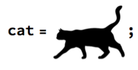
To convert a bitmap to a mesh first negate the color then use ImageMesh[] instead of DiscretizeGraphics[]:
catMesh=ImageMesh[ColorNegate[cat]]
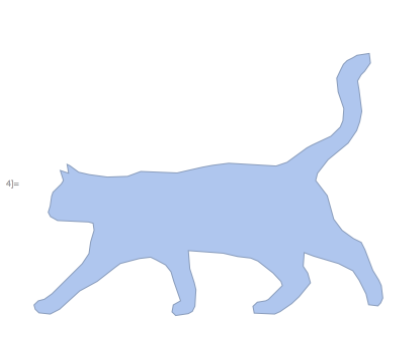
Next, you need to scale the image:
scaledCat = RegionResize[catMesh, {{-.8, .8}, {-.6, .6}}]

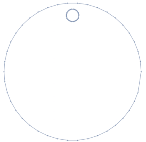
Lets use a disk for the base. Youll need to convert it to a mesh and make it slightly larger than 1 unit. (Remember you just scaled your image to be slightly smaller than the unit length:
base = DiscretizeGraphics[Graphics[{Disk[{0, 0}, 1.1]}]]

Lets make a hole in the base:
hole = DiscretizeGraphics[Graphics[{Disk[{0, .9}, .1]}]]
To make sure everything fits:
Show[{base, hole, scaledCat}, PlotRange -> All]

Lets first make the hole in the base:
base = RegionDifference[base, hole]

Now find the intersection:
intersection=RegionDifference[base, scaledCat]

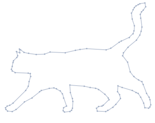
Now you need to get the boundary of the 2D mesh:
bdryCat = RegionBoundary[scaledCat]
bdryBase = RegionBoundary[base]
Create the levels:
level0 = 0.;
level1 = 0.15;
level2 = 0.25;
And now to put it all together:
Show[{
 RegionProduct[base, Point[{{level0}}]],
 RegionProduct[bdryBase, Line[{{level0}, {level1}}]],
 RegionProduct[intersection, Point[{{level1}}]],
 RegionProduct[bdryCat, Line[{{level1}, {level2}}]],
 RegionProduct[scaledCat, Point[{{level2}}]]
 }]
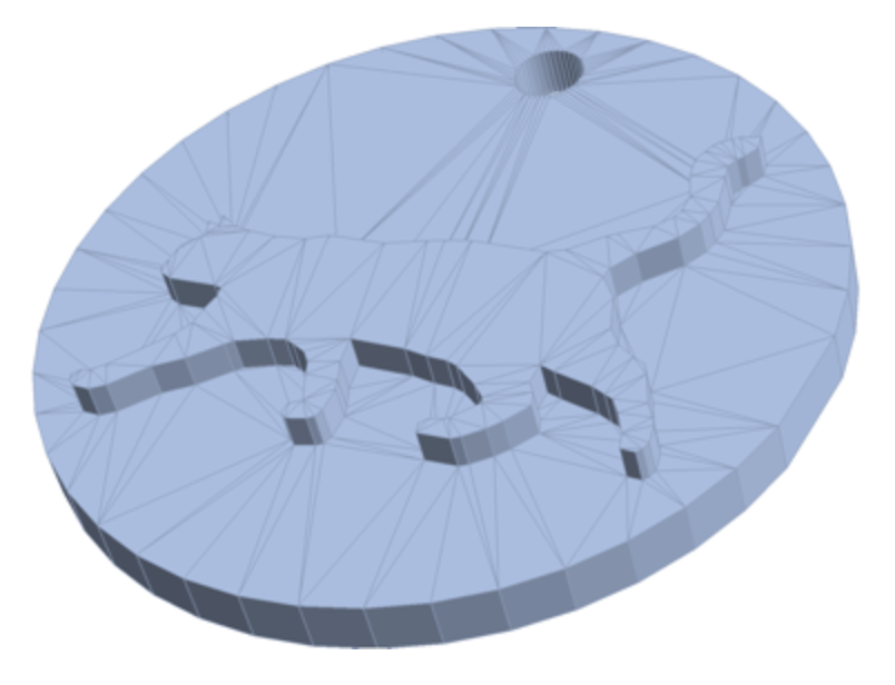
Export and print!
There you have it: a name tag in Mathematica. Not only did you get to learn a little about Mathematica, but you also got to see how meshes from two shapes are constructed. Where does Mathematica and 3D printing fit in the curriculum? Math class is an obvious answer, but its also well suited for a programming class, and with access to computers, patience and time, why not bring Mathematica and 3D printing to the art studio?
Heres a challenge: Try Mathematica for 15 days and see what you can do with it. Upload your 3D models to Youmagine and tag them #MathematicaAnd3DPrinting.


