Message Boards Message Boards

[?] Plot a Numerical Integration of (0.00159155/(x^2 + 0.000025^2))?

Posted 6 years ago

I have been Numerically Integrating the function (0.00159155/(x^2 + 0.000025^2)) from -10 to 10. But what i get is the ordinate values and when i plot it, it just shows the ordinate plot. Any way i can use array options from -10 to 10, show the integral values in a table and then list plot it?

Attachments:
POSTED BY: Mujtaba Mozumder
19 Replies

Right. Thanks.

POSTED BY: Mujtaba Mozumder

ok

POSTED BY: Mujtaba Mozumder

I got it right out of the notebook you posted.

Please stop taking this thread in circles.

POSTED BY: Daniel Lichtblau

@Mujtaba Mozumder have you noticed how people format code in comments here? Have you read the rules we linked for you http://wolfr.am/READ-1ST ?

The rules explain how to format your code properly. If you do not format code, it may become corrupted and useless to other members. Please EDIT your posts and make sure code blocks start on a new paragraph and look framed and colored like this.

int = Integrate[1/(x^3 - 1), x];
Map[Framed, int, Infinity]

enter image description here

POSTED BY: Moderation Team

The integrand code that you gave

{int, {evals}} = Reap[NIntegrate[ 0.00159155/(x^2 + 0.0000001 x + 0.000025^2), {x, -10, 10}, Method -> {"TrapezoidalRule", "Points" -> 100, "RombergQuadrature" -> False}, EvaluationMonitor :> Sow[{x, 0.00159155/(x^2 + 0.0000001 x + 0.000025^2)}, "EVAL"], MaxRecursion -> 0] // Quiet, {"EVAL"}];

has the function 0.00159155/(x^2 + 0.0000001 x + 0.000025^2) but i originally gave the function 0.00159155/(x^2+ 0.000025^2). Can you explain why you added 0.0000001 x ?

POSTED BY: Mujtaba Mozumder

Ok got it. Thank you for the explanations and details :)

POSTED BY: Mujtaba Mozumder

(1) It's not divergent. An approximation to a delta function cannot be divergent.

(2) You already have a way to do that area summation. It was in the original post, using NIntegrate.

(3) Your approximate delta function is actually off by a constant factor of around 200 (I assume you knew this but belaboring the detail regardless). The actual unmodified approximation would be alpha/Pi*1/(x^2+alpha^2). It is easy to see how this is related to the variant used in these posts.

alf = 0.000025;
numerator = 0.00159155;
multiplier = numerator/(alf/Pi)

(* Out[79]= 200.000071513 *)

So yours is larger by a factor quite close to 200. Easy to check that this is what is seem in the summation. Recall that integrating a good approximation to a delta function across the origin should give something very close to unity. So we expect your integral to be very close to 200.

NIntegrate[(numerator/(x^2 + alf^2)), {x, -10, 10}]

(* Out[80]= 199.999753203 *)

This can be done as an exact integral by the way.

exact = 
 Integrate[(1/(x^2 + alf1^2)), {x, -10, 10}, Assumptions -> alf1 > 0]

(* Out[85]= (2 ArcTan[10/alf1])/alf1 *)

Now evaluate numerically with substituted value for alf1 and the constant factor restored.

numerator*exact /. alf1 -> alf

(* Out[87]= 199.999753203 *)
POSTED BY: Daniel Lichtblau

Since it is divergent, is there a way i can find out the area under the curve by dividing it into arrays or trapezoids, taking many very small approximations and then combine the overall result?

Attachments:
POSTED BY: Mujtaba Mozumder

(It's really an approximation to the delta "function"). The plot shows a function that is small away from zero, and rises sharply at zero. If you use the option ListPlot[Sort[evals[[1]]], PlotRange->All] then you get a different scale to account for the peak as well as valley, and it looks like a straight line at zero. Squint hard and you see a lone dot at the origin, where it spikes.

All of which is in line with what one might expect for a plot of a function that numerically behaves as an approximation to the delta functional (to call it by the technically correct term).

POSTED BY: Daniel Lichtblau

Thank you. Sorry being unclear, plotting Dirac Delta function in Mathematica is actually very confusing for me. Can't understand what the plot actually is showing

Attachments:
POSTED BY: Mujtaba Mozumder

Which means the integrand will be close to zero away from the origin and will have a spike near the origin.

Your code:

{int, {evals}} = 
  Reap[NIntegrate[
     0.00159155/(x^2 + 0.0000001 x + 0.000025^2), {x, -10, 10}, 
     Method -> {"TrapezoidalRule", "Points" -> 100, 
       "RombergQuadrature" -> False}, 
     EvaluationMonitor :> 
      Sow[{x, 0.00159155/(x^2 + 0.0000001 x + 0.000025^2)}, "EVAL"], 
     MaxRecursion -> 0] // Quiet, {"EVAL"}];

Plot it:

ListPlot[Sort[evals[[1]]]]

You will see something along the lines described above.

The integral from -10 to T, where T ranges to +10, will look approximately like the Heaviside theta function (and I showed that in a prior response).

It would be good to figure out what it is you actually want, and then to state a clear question. As it is, responses are dealing with what seems to be a shifting landscape. Which may explain why a related question on Stack Exchange (which should have had cross-links) was closed.

POSTED BY: Daniel Lichtblau

also the function that i am using (0.00159155/(x^2 + 0.000025^2)) is a Dirac Delta function. I have attached a reference paper, currently using equation 5, assuming ? as 0.000025

Attachments:
POSTED BY: Mujtaba Mozumder

Sorry if i am being very unclear. Will the plotting graph for integral value and integrand be the same or different? Can you show me one for the integrand?

POSTED BY: Mujtaba Mozumder

Which Table? There are two in my answer.

t is the ABSCISSA, and int[t] is the INTEGRAL value. Now you ask about the INTEGRAND values, but you originally asked for only the INTEGRAL values. Which do you want?

POSTED BY: Michael Rogers

Thank you for your suggestion! Trying to work out if it is the INTEGRAND values that was plotted.

POSTED BY: Mujtaba Mozumder

My apologies. I couldn't find the previous thread. I worked out what you showed me. One thing that i am confused is, is the table we created showing the ORDINATE values or the INTEGRAND values? Trying to figure that out. Thank you for your suggestions!

POSTED BY: Mujtaba Mozumder

@Mujtaba Mozumder please do not duplicate discussions, this is against the rules: http://wolfr.am/READ-1ST

Your first thread is deleted and this one is kept. Please keep the same discussions contained in a single thread in future.

POSTED BY: Moderation Team

This seems to be the same question as http://community.wolfram.com/groups/-/m/t/1250846

You didn't reply to my answer, in which I showed how to make a table of values. I assumed you knew how to ListPlot it. You could also Plot[int[t], {t, -10, 10}] it.

And you could symbolically integrate it.


MOD TEAM NOTE: Original post mentioned here:

If you mean find $\int_0^t (0.00159155/(x^2 + 0.000025^2)) \; dx$ for various values of $t \in [-10, 10]$, then first use NDSolve to find an indefinite integral:

int = NDSolveValue[{y'[x] == (0.00159155/(x^2 + 0.000025^2)), y[0] == 0}, y, {x, -10, 10}]

and then make a Table:

Table[{t, int[t]}, {t, -10, 10, 0.1}]

Or for just the values:

Table[int[t], {t, -10, 10, 0.1}]
POSTED BY: Michael Rogers

If I understand correctly, you can get a Riemann approximation to what you want just by taking partial sums with Accumulate.

ListPlot[Transpose[{evals[[1, All, 1]], Accumulate[evals[[1, All, 2]]]}]]

This is not so accurate though. Perhaps better, if somewhat cumbersome, is to gather the sampling points as you already do, order them, then redo the integrations between consecutuve pairs thereof. Accumulating these subinterval integrals will give the picture I think you are after. Here is the idea.

(* repeat code from original post *)
rulePoints = 5;
sampledPoints = 
  Reap[NIntegrate[(0.00159155/(x^2 + 0.000025^2)), {x, -10, 10}, 
     Method -> {"LocalAdaptive", "SymbolicProcessing" -> 0, 
       Method -> {"TrapezoidalRule", "Points" -> rulePoints}, 
       "SingularityHandler" -> None}, EvaluationMonitor :> Sow[x]]][[2, 1]];

(* Now integrate between sampled points *)
newpoints = Sort[sampledPoints];
ivals = Table[NIntegrate[(0.00159155/(x^2 + 0.000025^2)), {x, newpoints[[i]], 
     newpoints[[i + 1]]}], {i, Length[newpoints] - 1}];

Plot:

ListPlot[Transpose[{Rest[newpoints], Accumulate[ivals]}], PlotRange -> All]
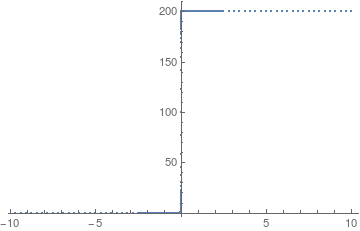
enter image description here

Maybe slightly better on the eyes:

ListPlot[Accumulate[ivals], PlotRange -> All]
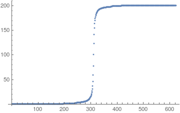
enter image description here

POSTED BY: Daniel Lichtblau
Reply to this discussion
Community posts can be styled and formatted using the Markdown syntax.
Reply Preview
Attachments
Remove
or Discard

Group Abstract Group Abstract