Touch ’Em All

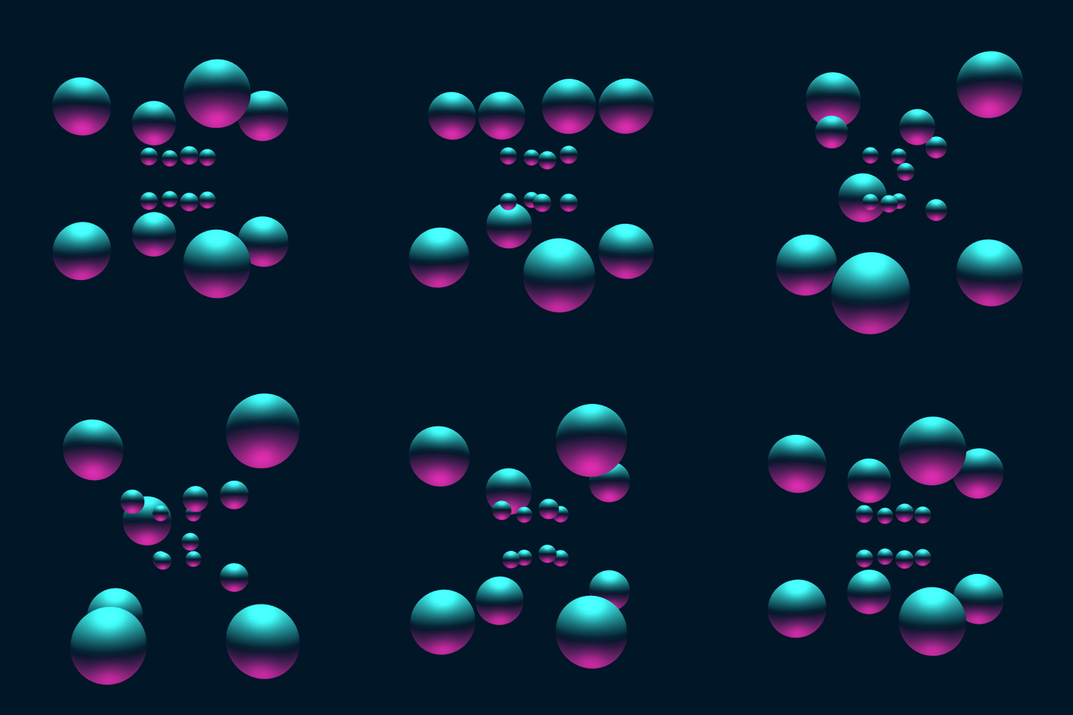
Consider the vertices of the hypercube as points on the 3-sphere. If we center a sphere of radius 0.2 at each vertex and stereographically project to $\mathbb{R}^3$, the result is the first frame in this animation.

Of course, to accomplish that we need a stereographic projection function:

Stereo[{x1_, y1_, x2_, y2_}] := {x1/(1 - y2), y1/(1 - y2), x2/(1 - y2)}

As well as the ProjectedSphere[] function from Inside (which I won't reproduce here due to its length and unpleasantness, but which produces the stereographic image of a given sphere in the 3-sphere).

Now, the animation shows a Hamiltonian cycle of the 1-skeleton of the hypercube (a.k.a., the hypercube graph). Now one can extract such a Hamiltonian cycle using FindHamiltonianCycle[HypercubeGraph[4]], but the coordinates of the vertices of HypercubeGraph[4] are only given in 2-D, so this doesn't help so much with actual visualization. So instead I construct the 1-skeleton of the hypercube, find a Hamiltonian cycle using FindHamiltonianCycle[], and then sort the vertices to appear in the order from the given cycle (by semi-coincidence, this actually turns out to be exactly the same Hamiltonian cycle as one gets from evaluating FindHamiltonianCycle[HypercubeGraph[4]]):

sortedHypercubeVertices = 
  Module[{v = Tuples[{1/2, -1/2}, {4}], M, G, cycle},
   M = Table[
     If[HammingDistance[v[[i]], v[[j]]] == 1, 1, 0],
     {i, 1, Length[v]}, {j, 1, Length[v]}];
   G = AdjacencyGraph[M];
   cycle = FindHamiltonianCycle[G];
   v[[#[[1]] & /@ (cycle[[1]] /. UndirectedEdge -> List)]]
   ];

With that all in place, then, we just need to rotate the $i$th vertex to the $(i+1)$st vertex (mod 16) up in the 3-sphere and then stereographically project (with a little help from the smoothstep function, which makes the transitions less jarring):

smoothstep[t_] := 3 t^2 - 2 t^3;

DynamicModule[{\[Theta], pts = N[sortedHypercubeVertices], 
  cols = RGBColor /@ {"#41EAD4", "#B91372", "#011627"}},
 Manipulate[
  \[Theta] = \[Pi]/3 smoothstep[t];
  Graphics3D[
   {Specularity[.4, 10],
    Table[
     ProjectedSphere[RotationMatrix[\[Theta], {pts[[i]], pts[[Mod[i + 1, Length[pts], 1]]]}].pts[[i]], .2],
     {i, 1, Length[pts]}]},
   PlotRange -> 3, Boxed -> False, ViewPoint -> 1/2 {2, 1, 0}, ViewAngle -> \[Pi]/4,
   Lighting -> {{"Directional", cols[[1]], {0, 0, 50}},
     {"Directional", cols[[2]], {0, 0, -50}},
     {"Ambient", cols[[-1]]}},
   Background -> cols[[-1]], ImageSize -> 540],
  {t, 0, 1}
  ]
 ]