The following is a notebook in the cloud (1 MB), that one can best download and run on the desktop (see the browser in the lower right). It has initialisation cells for two small packages.
https://www.wolframcloud.com/objects/thomas-cool/Voting/2018-01-18-Aitchison.nb
Readers who recently looked at the Brexit discussion will find the topic familiar, see
http://community.wolfram.com/groups/-/m/t/1221950
The summary of the notebook is:
Votes and seats satisfy only two of seven criteria for application of the Aitchison distance. Vectors of votes and seats, say for elections for political parties the House of Representatives, can be normalised to 1 or 100%, and then have the outward appearance of compositional data. The Aitchison geometry and distance for compositional data then might be considered for votes and seats too. However, there is an essential zero when a party gets votes but doesn't gain a seat, and a zero gives an undefined logratio. In geology, changing from weights to volumes affects the percentages but not the Aitchison distance. For votes and seats there are no different scales or densities per party component however, and thus reportioning (perturbation) would be improper. Another key issue is subcompositional dominance. For votes {10, 20, 70} and seats {20, 10, 70} it is essential that we consider three parties. For a disproportionality measure we would value it positively that there is a match on 70. The Aitchison distance looks at the ratio {10, 20, 70} / {20, 10, 70} = {1/2, 2, 1} and then neglects a ratio equal to 1. In this case it essentially compares the subcompositions, i.e. votes {10, 20} and seats {20, 10}, rescales to {1/3, 2/3} and {2/3, 1/3}, and finds high disproportionality. This means that it essentially looks at a two party outcome instead of a three party outcome. It follows that votes and seats are better served by another distance measure. Suggested is the angular distance and the Sine-Diagonal Inequality / Disproportionality (SDID) measure based upon this. Users may of course apply both the angular and the Aitchison measures while being aware of the crucial differences in properties.
NB. This discussion forms part of a larger framework given most recently by my other paper: "One woman, one vote. Though not in the USA, UK and France". My diagnosis is that "political science on electoral systems" is still in the Humanities and pre-science, notably by relying more upon common language instead of sharp definitions that are relevant for empirics. On the other hand, there are also mathematicians who deal with their definitions abstractly, without a proper grounding in empirical research. My invitation to empirical researchers is to help make a difference, notably in re-engineering the theory on electoral systems.
1. Introduction
Content and didactics
This paper solves an issue on content and employs some didactics to do so.
On content: Votes and seats satisfy only two out of seven criteria for application of the Aitchison distance. It follows that votes and seats are better served by another distance measure, notably the angular distance and its transforms. Nevertheless, the Aitchison geometry might be a useful environment for the analysis of compositional data, and thus we should be aware of the properties.
On didactics: Mathematics provides clear definitions of improduct, norm and distance, and we are familiar with them for Euclidean space. When we apply these notions to different spaces then we find that understanding becomes still complicated. Especially education is challenged on those concepts for different spaces. It appears that Mathematica allows us to better grasp the issues. Mathematica is a system for doing mathematics on the computer. It allows the combination of texts, symbols, numbers, graphs, patterns, motion, sound, etcetera. The following application to the Aitchison geometry again shows the power of using this integrated system.
Three spaces and compositional data
We consider three spaces:
(1) the original Euclidean space with vectors (of votes and seats) x [GreaterSlantEqual] 0
(2) the space with shifted logratio Log[(x + 1) / (y + 1)]
(3) the space with centered logratio Log[x / g[x]], with y = g[x] the geometric mean.
We first review the notions of improduct, norm and distance for Euclidean space.
Subsequently we introduce the notion of compositional data: vectors x > 0 such that 1'x = 1, or that the sum of the components add up to 1. These vectors are in the unit simplex, or, the endpoints of the vectors are onto the plane that characterises the unit simplex. Potentially some components might be zero, and these might be neglected unless there are essential zeros.
Our target application concerns votes and seats. For example, the outcomes for Parties A and B might be votes = {49, 51} and seats = {51, 49}, both in percentages. Those votes and seats are compositional data, at least in outward appearance. We would be interested in a measure of distance between these two outcomes.
Political science on electoral systems has provided various measures of distance, of which we will mention the two main ones: The Loosemore-Hanby measure is based upon the absolute difference (ALHID) and the Gallagher measure is based upon the Euclidean distance (EGID), both with corrections to get an outcome in [0, 1], [0, 10] or [0, 100] depending upon the preferences of the researcher. It appears that these measures have some drawbacks. My suggestion from econometrics and political economy is to use the angle between the vectors, which in particular gives the transformation into the Sine-Diagonal Inequality / Disproportionality (SDID), see Colignatus (2017ac). For this present notebook it suffices to use a simpler indicator. Since the maximum angle between nonnegative vectors is 90 degrees, we can interprete the angle also as share of 90 degrees, henceforth AngularID.
The motivation for this notebook is that we should not overlook the suggestion of the Aitchison distance for compositional data. This notebook first discusses this geometry so that we understand its key properties. The two penultimate sections discuss the relevance of the Aitchison geometry for votes and seats. The conclusion is that the Aitchison geometry is less suited for a disproportionality measure for votes and seats. Obviously we may use both measures as long as we understand the properties.
Comparing votes and seats is a topic of its own
For compositional data, the ratios Subscript[x, i] / Subscript[x, j] are regarded as generating more relevant information than the absolute values. Aitchison (1926-2016) proposed the "log-ratio" approach, using Log[Subscript[x, i] / Subscript[x, j]] = Log[Subscript[x, i]] - Log[Subscript[x, j]] as the relevant measurement, corrected for the geometric means. The centered logratio approach essentially switches to the log of the ratio to the geometric average, and then applies the distance notions of the Euclidean space to those. To do so, however, still requires some essential understanding of geometry. Researchers in a particular field of interest obviously must understand what the transformations imply for the field of interest.
For proper compositional data and their analysis, it appears that the centered logratio transformation is more important than the phenomenon that the data can be seen as being on the unit simplex. The conclusion of this present discussion may also be summarized as that the centered logratio transformation is inadequate for comparing votes and seats.
It appears that Aitchison has actually two different lines of analysis. The first line is that compositional data add up to the unit simplex, the second line is the logratio transform. It is important to be aware that the latter transforms are not on the unit simplex. For example, when we have a vector of vote shares {1, 1.5, 2.5, 5} on a scale of 10, then the centered logratio transform gives the following vector, and adding it generates 0 instead of 1.
CenteredLogRatio[{1, 1.5, 2.5, 5}]
{-0.732798, -0.327333, 0.183492, 0.876639}
% // Total // Chop
0
The implication of compositional data is that we lose a degree of freedom, and that we should drop one variable since it is explained by the summation. However, when we compare votes and seats then we would not drop a variable since we also want to take account of the deviation there.
For the literature on compositional data, it would be useful to distinguish between cases where the Aitchison geometry applies and those where it doesn't apply. Perhaps it might suffice to say that the criterion of being on the unit simplex is not enough to count as proper compositional data, so that votes and seats are only pseudo-compositional data. However, the main insight would rather be that the comparison of votes and seats would be a different kind of analysis than merely using a particular space.
While this present discussion is within the overlap of political economy with political science on electoral systems, we may refer to the econometrics literature, notably Theil (1971:628) on the probit and logit models, and to Cramer (1975:204) who uses the centered logratio: "First we adopt the almost universal usage of taking logarithms of price and quantity (...) We also suppress the constant terms in all relations by taking deviates from the sample mean (...) of logarithms." The latter is using the centered logratio approach. This present paper only doubts the relevance of the logratio transform for establishing the distance between votes and seats. Section 10 below will look at approaches in political science of estimating and predicting votes, which is another issue than comparing votes and seats.
Another element of didactics
For didactic reasons, we look first at an intermediate model that allows us to better grasp what Aitchison does. This approach uses the transform Log[x + 1] ? x, which approximation is fairly good for values of x ? 0. The addition of 1 moves the vector upwards but the logarithm moves it back towards the origin. We then look at the revised ratio Log[(Subscript[x, i] + 1) / (Subscript[x, j] + 1)] = Log[Subscript[x, i] + 1] - Log[Subscript[x, j] + 1] ? Subscript[x, i] - Subscript[x, j]. This has both a notion of a ratio and outcomes similar to the absolute values. For example, comparing 10% to 5%, then Log[10/5] = Log[2] ? 70% while Log[1.1 / 1.05] ? 5%. This didactic setup allows us to get used to the notion of a ratio and the log transform, and repeats the triad of improduct, norm and distance, so that we get a better feel for that triad. This approach however fails for votes and seats because there is no real departure from the absolute levels, and thus it suffers the same drawbacks as the Loosemore-Hanby and Gallagher measures. Comparing this Log[x + 1] transform with the Aitchison approach shows that the latter deals much better with the ratios, so that we are more motivated to understand what the Aitchison geometry is.
Technical
This notebook uses v for votes, s for seats, V = 1'v for the sum of votes, S = 1's for the sum of seats, w = v / V, z = s / S for the shares. The plots tend to use opposite formulas, as z = 1 - w, using z = {t, 1 - t}, with t for the seats of the first party. For votes and seats we prefer a normalisation to [0, 10], given that [0, 1] causes leading zeros and [0, 100] suggests precision that is often lacking.
PM. The Appendix E in the original version of this paper was split off as an independent text, Colignatus (2018). There is now also a stricter scaling of votes and seats into the [0, Ð] range, default Ð = 10 (see Section 4). Chapter 10 discusses some papers in the voting literature that have referred to the Aitchison analysis, but that do not compare votes and seats.
NB. This discussion forms part of a larger framework given most recently by Colignatus (2017b): "One woman, one vote. Though not in the USA, UK and France". My diagnosis is that "political science on electoral systems" is still in the Humanities and pre-science, notably by relying more upon common language instead of sharp definitions that are relevant for empirics. On the other hand, there are also mathematicians who deal with their definitions abstractly, without a proper grounding in empirical research. My invitation to empirical researchers is to help make a difference, notably in re-engineering the theory on electoral systems.
Routines in this notebook
?Cool`Statistics`Aitchison`*

?Cool`Voting`Angular`*

2. Euclidean improduct, norm, distance and angle
Pythagoras, length and size
In Mathematica, Dimensions[x] gives the list of dimensions of x. For a vector x, Length[x] gives the number of components.
{Dimensions[{a, b, c}], Length[{a, b, c}]}
{{3}, 3}
The Pythagorean Theorem allows us to find the size length of a vector. Another name is the norm || x ||. Mathematica assumes complex vectors and thus uses Abs[x] for the size of the components. Since we use real vectors, we may eliminate this Abs.
?Norm
Norm[{a, b, c}]
% /. Abs -> Identity

The triad of improduct, norm and distance
Consider the steps: improduct -> norm -> distance.
In Euclidean space, the improduct is given as the Dot product x . y. In linear algebra we write x' y.
?Dot

{a, b, c} . {x, y, z}
a x + b y + c z
For variables in real space, the norm of x amounts to application of the improduct to x and itself, and then taking the square root.
Norm[{a, b, c}] == Sqrt[{a, b, c} . {a, b, c}]

The distance between vectors x and y is given as the norm of their difference. We look at real vectors, and eliminate Abs.
Norm[{a, b, c} - {x, y, z}] /. Abs -> Identity

EuclideanDistance[{a, b, c}, {x, y, z}] /. Abs -> Identity
Invariance to translation
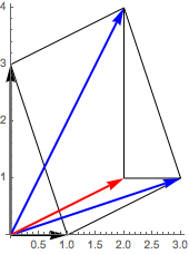
A translation is an additive relocation by some z. The distance between x and y is unaffected by a translation to x + z and y + z. This is easy to prove: Norm[(x + z) - (y + z)] = Norm[x - y]. The following shows the translation of two (black) vectors by z = {2, 1} (red) giving two translated (blue) arrows.
org = {0, 0}; pa = {0, 3}; pb = {1, 0}; pat = pa + {2, 1}; pbt = pb + {2, 1};
lin1 = Line[{pa, pat, pbt, pb, pa}];  lin2 = Line[{pat, {2, 1}, pbt}];
arpa = Arrow[{org, pa}]; arpat = Arrow[{org, pat}];
arpb =  Arrow[{org, pb}]; arpbt = Arrow[{org, pbt}];
arpz = Arrow[{org, {2, 1}}];
Graphics[{lin1, lin2, Thick, Arrowheads[.1], arpa, arpb, Blue, arpat, arpbt,
  Red, arpz }, Axes -> True, AspectRatio -> Automatic]
Subspace dominance
The size of vectors is always larger than their parts in subspaces. This is called subspace dominance.
Formally, dist[s1, s2] ? dist[x1, x2] when s1 and s2 are in the same subspaces of x1 and x2.
Consider:
x1 = {.1, .2, .7};
s1 = Drop[x1, -1];
x2 = {.2, .1, .7};
s2 = Drop[x2, -1];
The final elements in x1 and x2 are the same, and this causes that x1 and x2 are as far apart as s1 and s2. When the final elements in x1 and x2 would differ, this would only increase the Euclidean distance.
{EuclideanDistance[x1, x2], EuclideanDistance[s1, s2]}
{0.141421, 0.141421}
When we use the Norm then we see a zero where the vectors have the same values. Adding a zero size length obviously does not affect the outcome of the Norm.
{Hold[Norm][x1 - x2], Hold[Norm][s1 - s2]}
{Hold[Norm][{-0.1, 0.1, 0.}], Hold[Norm][{-0.1, 0.1}]}
% // ReleaseHold
{0.141421, 0.141421}
Metric
Given the properties of the Euclidean norm, the Euclidean distance d is a metric.
A distance d is a metric iff it satisfies these three properties:
(1) d[x, y] ? 0, and d[x, y] = 0 iff x = y
(2) Symmetry: d[x, y] = d[y, x]
(3) The triangular inequality: d[x, z] ? d[x, y] + d[y, z] for y other than x or z.
Angle and its estimate
Two vectors always form a plane. Improduct and norm allow us to define the cosine of an angle between vectors.
Cos[?] = Cos[x, y] = x . y / ( ||x|| ||y|| ) = Improduct[x, y] / (Norm[x] Norm[y]).
The angle itself can be found by the inverse of the cosine, as ? = ArcCos[Cos[?]].
?VectorAngle

The angle distance is a metric. The "cosine distance" 1 - Cos[x, y] is not a metric because it does not satisfy the triangular inequality, see Van Dongen & Enright (2012).
Mathematica assumes complex variables, and thus its internal definition of the vector angle uses Abs and Conjugate. We can eliminate this however. We also look at nonnegative vectors, for which the maximum angle is 90 degrees. We get a relative measure of angular distance when we divide the angle by this maximum. We already showed this in the Introduction in numbers but let us repeat it here in symbols.
VectorAngle[{a, b, c}, {d, e, f}] /. {Abs -> Identity, Conjugate -> Identity}
The AngularID (AID) scales to [0, Ð], default Ð = 10. Thus, an AID outcome h stands for 90 h / 10 = 9 h degrees of the angle between the vectors.
?AngularID

The angular distance is independent from any positive scalar multiple per vector.
Simplify[AngularID[ ? {a, b, c}, ? {d, e, f}] == AngularID[{a, b, c}, {d, e, f}], {? > 0, ? > 0}]
True
Appendix B shows an approximation of the angle ? ? || x / ||x|| - y / ||y|| ||, which works good for small angles.
3. Theoretical requirements for a norm
It is useful to state the theoretical requirements of a norm, so that we can use these also for the Aitchison geometry.
A norm requires a vector space.
Definition of a vector space
A vector space has both vector addition and scalar multiplication.
(A) Addition has:
(1) Symmetry / commutativity: x + y = y + x
(2) Associativity: x + (y + z) = (x + y) + z
(3) There is a neutral or identity element 0, such that x + 0 = x
(4) Each element x has an inverse, denoted -x, such that x + (-x) = 0
(B) For scalar multiples ? and ?:
(1) Associativity: ? (? x) = (? ?) x
(2) There is a neutral or identity element ? = 1, such that ? x = x
(3) Distributivity 1: ? (x + y) = ? x + ? y
(4) Distributivity 2: (? + ?) x = ? x + ? x
Definition of a norm
When there is a vector space V, then the definition of a norm norm: V -> Reals is:
(1) Homogeneity or absolutely scalable: norm[? x] = Abs[?] norm[x]
(2) Subadditive or triangular inequality: norm[x + y] <= norm[x] + norm[y]
(3) Nonnegative: norm[x] ? 0
(4) Definite: norm[x] = 0 iff x = 0
When distance d[x, y] = norm[x - y] then the homogeneity of the norm gives d[? x, ? y] = Abs[?] d[x, y]
4. Inequality / disproportionality measures of votes and seats
This section is essentially copied from Colignatus (2018).
Normalisation to 10 rather than 1 or 100
For political science there is the choice between training students to grow sensitive to small numbers or create more sensitive measures that also allow direct communication with the larger public. For the Richter scale for earthquakes, the approach was to use logarithms, so that smaller values could be compared easier with larger ones. For our purposes the square root is adequate, with an easy change from 10 (grade) to 100 (percentage).
For this subject of votes and seats it is better to use the grades in [0, 10], like votes = {4.9, 5.1}. The reason is that variables in [0, 1] causes leading zeros, while percentages in the range [0, 100] suggest a degree of precision that is often overdone.
For the scale we will use the symbol Ð (capital eth). For example w = Ð v / V. The default value in this paper is Ð = 10.
?UnitÐ
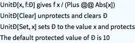
?Ð

UnitÐ[{49, 51}] // N
{4.9, 5.1}
1 / Ð == 10 Percent
1/10 == 10 Percent
Data of the US House of Representatives elections of 2016
It will be useful to have some example. At the US (half) elections of 2016 for the House of Representatives, the distributions for the votes and seats were, using the order {Democrats, Republicans, Other}:
votes = {dem = 61776554, rep = 63173815, 128627010 - rep - dem};
seats = {194, 241, 0};
The operation of "closure" divides a vector by its sum total.
?Closure

For votes we prefer to use UnitÐ.
{vts = UnitÐ[votes], sts = UnitÐ[seats]} // N
{{4.80277, 4.9114, 0.285837}, {4.45977, 5.54023, 0.}}
Show[ListLinePlot[{{0, 0}, 6 {1, 1}}],
 ListPlot[MapThread[Labeled, {Transpose[{vts, sts}], {Dem, Rep, Other}}],
  PlotStyle -> PointSize[Large]], AxesLabel -> {"Votes (Ð)", "Seats (Ð)"},
 AspectRatio -> 1]
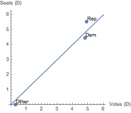
The USA have district representation which differs from equal or proportional representation (like in Holland). In a US district, a candidate is elected with the plurality rule. The votes for other candidates than the winner are discarded. That the Democrats and Republicans are still relatively close to the 45 Degree line of equality or proportionality is the effect of geography, and perhaps the median voter theorem. The word "election" is over-used when it refers to such different meanings for either district or proportional representation. Given the discarding of votes in the system of district representation, we rather should speak about "half elections".
In district representation, there will also be more strategic voting, in which voters will not vote for a smaller party for fear that their vote will be discarded. This effect cannot be measured by the common inequality or disproportionality measures, since we only have the recorded votes and not the true preferences.
Disproportionality measures
The common notion is distance but for votes and seats we would like to see equal proportions, whence we also speak about an inequality / disproportionality (ID) measure.
The following measures are used in the literature on votes and seats, with the sine-diagonal measure a new suggestion from 2017. The measures are all symmetric, except Webster / Sainte-Laguë.
The literature uses values of ALHID and EGID in the [0, 100] range. We use the [0, 10] range here.
AbsLoosemoreHanbyID (ALHID)
?AbsLoosemoreHanbyID

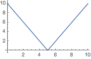
Plot[AbsLoosemoreHanbyID[{Ð - t, t}, {t, Ð - t}], {t, 0, Ð}]
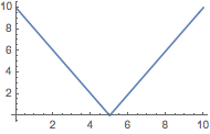
The LHID measure has the useful interpretation that it gives the share of displaced seats between parties for a House of Ð seats (corrected for double counting). In the US, 0.6 seats of a House of 10 seats are displaced, or 6 in a House of 100 seats.
AbsLoosemoreHanbyID[votes, seats] // N
0.628834
The ALHID distance is insensitive to the location of a 1 grade difference, say at {4, 6} or {9, 1}.
{ad1 = AbsLoosemoreHanbyID[{4, 6}, {5, 5}],
  ad2 = AbsLoosemoreHanbyID[{9, 1}, {10, 0}], ad1/ad2} // N
{1., 1., 1.}
EuclidGallagherID (EGID)
?EuclidGallagherID

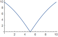
Plot[EuclidGallagherID[{Ð - t, t}, {t, Ð - t}], {t, 0, Ð}]
The 2016 US House data have 3 parties, and thus the EGID can have a different outcome than the ALHID. The US EGID is a bit larger than a half grade or 5%.
EuclidGallagherID[votes, seats] // N
0.545336
For two parties, the insensitivity is the same for EGID as ALHID.
{ad1 = EuclidGallagherID[{4, 6}, {5, 5}],
  ad2 = EuclidGallagherID[{9, 1}, {10, 0}], ad1/ad2} // N
{1., 1., 1.}
Angular inequality / disproportionality (AID)
?AngularID

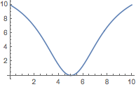
Plot[AngularID[{Ð - t, t}, {t, Ð - t}], {t, 0, Ð}]
The 2016 US AID would suggest a disproportionality in the USA of 0.7 grades or 7%.
AngularID[votes, seats] // N
0.66848
The angular distance is sensitive to the location of 1 grade difference. It shows a halving or doubling of the angular distance, depending where one starts.
{ad1 = AngularID[{4, 6}, {5, 5}],
  ad2 = AngularID[{9, 1}, {10, 0}], ad1/ad2} // N
{1.25666, 0.704466, 1.78385}
Because of this greater sensitivity the angular distance is a better measure for disproportionality than ALHID and EGID.
Sine-Diagonal (SDID)
?SineDiagonalID
 If we do not look at input of opposites.
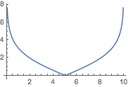
Plot[SineDiagonalID[{50, 50}, {t, Ð - t}], {t, 0, Ð}]
The input of opposites generates negative outcomes, indicating majority switches between votes and seats.
Plot[SineDiagonalID[{Ð - t, t}, {t, Ð - t}], {t, 0, Ð}]
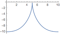
The SDID measure is designed to be sensitive to disproportionality. For the US it gives 3.2 on a scale of 10, thus 32%. The SDID uses a magnifying glass like the scale of Richter on earthquakes does. (Smaller earthquakes are made comparable with the bigger ones.)
SineDiagonalID[votes, seats] // N
3.23746
The SDID is steeper than the AID, which makes the ratio of inner versus outer range values for the displacement a bit lower.
{ad1 = SineDiagonalID[{4, 6}, {5, 5}],
  ad2 = SineDiagonalID[{9, 1}, {10, 0}], ad1/ad2}// N
{4.4285, 3.32312, 1.33263}
Webster / Sainte-Laguë (WSLID)
The measure is sensitive to ratios and without bound, so there is no real criterion to judge what an outcome really means.
?WebsterSainteLagueID

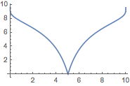
Plot[WebsterSainteLagueID[{Ð - t, t}, {t, Ð - t}], {t, 0, Ð}]
WebsterSainteLagueID[votes, seats] // N
0.390846
When a distance d has no upper value then it may always be transformed into Ð d / (1 + d) to get a value in [0, Ð) if needed.
Plot[(d = WebsterSainteLagueID[{Ð - t, t}, {t, Ð - t}] / Ð ;
  Ð  d / (1 + d)), {t, 0, Ð}]
The Aitchison distance
Though we haven't defined the Aitchison distance here yet, we may already calculate and plot it with the same input as above.
?AitchisonDistance

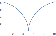
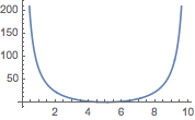
Plot[AitchisonDistance[{Ð - t, t}, {t, Ð - t}], {t, 0, Ð}]
It is difficult to judge an outcome when there is no frame of reference. When a distance d has no upper value then it may always be transformed into Ð d / (1 + d) to get a value in [0, Ð) if needed. It itself this plot of the Aitchison distance suggests that it might be used, but below we will look at various properties that are awkward for votes and seats.
Limit[AitchisonDistance[{1 - t, t}, {t, 1 - t}], t -> 0]
?
Plot[(d = AitchisonDistance[{Ð - t, t}, {t, Ð - t}]; Ð d / (1 + d)), {t, 0, Ð}]
For the US data, the Aitchison distance is undefined when there is a zero. Let us drop that case.
AitchisonDistance[Drop[votes, -1], Drop[seats, -1]] // N
0.137584
Appendix D discusses the relation between the Aitchison distance and the Webster / Sainte-Laguë inequality / disproportionality measure.
5. Compositional data
The unit simplex, closure and the neutral element
Compositional data are positive and their sum adds up to 1. Zeros would be eliminated, and all are divided by a constant.
The operation of "closure" divides a vector by its sum value.
?Closure

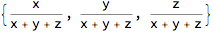
Closure[{x, y, z}]
This means that all vectors are projected onto the unit simplex.
?Simplex

Since we will be looking at logarithms and Log[1] = 0, there is a special role for the unit vector {1, 1, ..., 1}.
The projection of {1, 1, ..., 1} onto the unit simplex is called "UnAit" here.
?UnAit
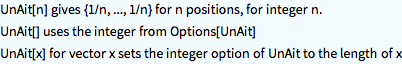
Options[UnAit]
{Integer -> 3}
UnAit[]
{1/3, 1/3, 1/3}
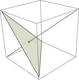
The following is an example from 3D, in which we project {1, 1, 1} onto the unit simplex and find {1, 1, 1} / 3.
zero = Table[0, {3}];
ones = Table[1, {3}];
simp = Simplex[{{1, 0, 0}, {0, 1, 0}, {0, 0, 1}}];
lin = Line[{ zero, ones }];
pnt = Point[ Closure[ones] ];
Graphics3D[{simp, lin, Red, PointSize[Large], pnt }]
The "ternary plot" is again a special transformation of the unit simplex for 3D.
Closure and angle
The angular distance is independent from closure, since this holds for any positive scalar multiple per vector.
As said we use the votes and seats of the US elections of 2016.
votes = {dem = 61776554, rep = 63173815, 128627010 - rep - dem};
seats = {194, 241, 0};
{vts = Closure[votes], sts = Closure[seats]} // N
{{0.480277, 0.49114, 0.0285837}, {0.445977, 0.554023, 0.}}
Closure is relevant for human understanding but not for the calculation of the angular distance, as this distance is unaffected by scalar multiples per vector.
{VectorAngle[votes, seats], VectorAngle[vts, sts]} / (90 Degree) // N
{0.066848, 0.066848}
The AngularID (AID) has been defined so that it scales into [0, Ð].
{AngularID[votes, seats], AngularID[vts, sts]} // N
{0.66848, 0.66848}
By comparison, to be discussed below, the Aitchison distance for American politics is, (i) depending upon our method to get rid of the zero, and (ii) without a reference like 100%:
AitchisonDistance[votes, seats + {0, -1, 1}] // N
2.07952
AitchisonDistance[Drop[votes, -1], Drop[seats, -1]] // N
0.137584
Practical cases and the essential zero
The notion of "Closure" may affect our perception of the data. We not only lose a degree of freedom. Aitchison has a strong argument that relative data are different from absolute data. The latter argument though seems more related to the use of the geometric mean than to closure, see below.
Examples of compositional data are:
(i) geology: soil, e.g. sand, biological materials, some water
(ii) biology: milk, e.g. fat, proteins, minerals, water (e.g. for different species like cows, cats, elephants, camels, ....}
(iii) politics: votes and seats for various political parties.
There are some distinctions between these kinds of compositional data however. On the following three aspects, votes and seats differ from the first two examples.
(1) For soil and milk, one can take many samples from various sources, but for elections we essentially compare a single outcome of votes with a single outcome of seats. It makes little sense to take an average of votes over various countries when the parties are quite different. Even for the same country and same parties, comparison over years causes us to compare votes and seats in each year apart, and it makes little sense to average the votes and seats separately, and then take the disproportionality of those constructs.
(2) For soil and milk, there might be no "essential zeros" while for seats there is the essential phenomenon that there can be votes for parties who gain no seats (collected in the category "other"). If we switch to logarithms, then Log[0] is undefined. NB. Parties that receive no votes may be neglected, as they would neither get seats.
(3) The underlying issue for votes and seats derives most meaning from apportionment in which the number of available seats S is important. With apportionment function Ap, we determine: seats = Ap[votes, S]. Thus S has a key role. Votes and seats have the outward appearance of compositional data but this should not cause us to infer that they share the other properties.
Aitchison's four criteria for distance
We can continue the list of aspects with four criteria on the distance measure (giving a total of seven criteria).
(4) Aitchison (undated), "Concise guide", p35, requires four properties of a compositional distance measure:
(a) scale invariance
(b) permutation invariance
(c) perturbation invariance (reportioning, componentwise rescaling)
(d) subcompositional dominance.
See also Martin-Fernandez et al. (undated) p2. The latter p3 show that the angular distance satisfies the first two properties but not the latter two. Thus, of the seven points considered here, votes and seats satisfy only two.
Comments on these criteria are:
(4a) Permutation invariance means that the political parties can be sorted in whatever manner.
(4b) For scaling: Votes and seats have a natural scale, namely the natural numbers, and the invariance to scale must only hold for the vectors as a whole: dividing the votes by turnout and dividing the seats by the number of seats in the House.
(4c) For reportioning (perturbation): This concerns different scales per component. For soil and milk, the components might be measured by weight or volume. If the components {x, y, z} are in volumes and the components have different densities {a, b, c}, or weights per volume, then {a x, b y, c z} would be the composition in weights. These formats would give different vectors by closure. For multiplicative factors, rescaling each component by its own factor (reportion or perturbation) is the equivalent of the (linear) translation in Euclidean geometry (see the diagram above for translation). For soil and milk it would be relevant that the outcome of the analysis does not depend upon weight or volume. For votes and seats there are no different scales per party component, and thus this does not apply. We discuss this further below.
(4d) We will look at subcompositional dominance below.
Spurious correlation
Karl Pearson (1857-1936) coined the term "spurious correlation" by referring to a particular case of compositional data. It appears that his example is somewhat convoluted, see Colignatus (2017d). The question is whether we correlate samples (rows) or components (columns). The term "spurious correlation" still is useful for when we have the wrong model and then find a correlation that does not reflect the true model. In the literature on compositional data, the reference to Pearson's discussion is somewhat popular, using a similarly convoluted example. If you consider soil samples, and compare the compositions of the original samples with the compositions of those that have been dried (with removal of the water), then one might get different correlations. It must be doubted however whether this particular setup for the correlations is so relevant, when there is a confusion of samples (rows) and components (columns). Overall, my impression is that neither the reference to Pearson nor this particular example of "spurious correlation" of soil compositions are so enlightening. It is one distraction that one has to look into though, when the literature refers to it.
6. Log Closure Plus One
Rebasing to Log[Closure[x] + 1]
This section shows how a log transform can create something similar to a distance that is sensitive to some ratio. The transforms cause properties that deviate from both Euclid and Aitchison. This is intended as a didactic step between Euclidean and Aitchison distance measures.
?LogClosurePlusOne

LogClosurePlusOne[{x, y, z}]
LogClosurePlusOne[{0, 1, 0}]
{0, 1, 0}
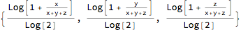
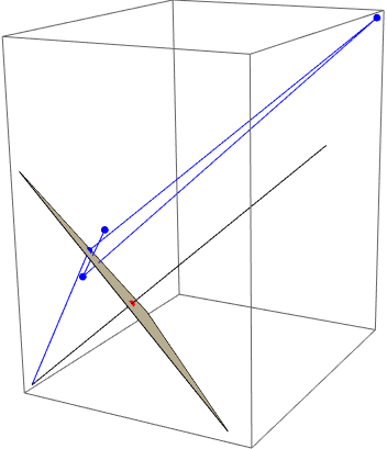
The transformation x + 1 maps x first with 1 to some "upper Simplex" beyond {1, 1, ..., 1}, and then Log projects back again. The following example uses co-ordinates cs = {.10, .35, .55} on the unit simplex. The blue line connects the origin to cs, to Closure[cs] + 1 = cs + 1, to Log[cs + 1], to Log[cs + 1] / Log[2]. See also the numerical output. The transformation will generate outcomes close to the unit simplex.
zero = Table[0, {3}];
ones = Table[1, {3}];
simp = Simplex[{{1, 0, 0}, {0, 1, 0}, {0, 0, 1}}];
lin = Line[{ zero, ones }];
pnt = Point[ Closure[ones]];
pnt1 = Point[{ cs = {.10, .35, .55}, cls = Closure[cs], cpo = cls + 1,
   lcpotrue = Log[cpo], lcpo = lcpotrue / Log[2] }]
lin1 = Line[{zero, cs, cls, cpo, lcpotrue, lcpo}];
Graphics3D[{simp, lin, Red, PointSize[Large],  pnt, Blue, pnt1, lin1 }]
Point[{{0.1, 0.35, 0.55}, {0.1, 0.35, 0.55}, {1.1, 1.35, 1.55}, {0.0953102, 0.300105, 0.438255}, {0.137504, 0.432959, 0.632268}}]
The triad of improduct, norm and distance
Following the model of Euclidean space, we need an improduct, norm and distance. We can employ the Euclidean definitions to the transformed data since these are still within Euclidean space.
?ImprodLCPO

ImprodLCPO[{a, b, c}, {d, e, f}]

?NormLCPO

NormLCPO[{a, b, c}]
?DistanceLCPO

DistanceLCPO[{a, b, c}, {d, e, f}]

DistanceLCPO[x, y] gives Norm[LCPO[x] - LCPO[y]]. The subtraction means that we use something similar to the logratio: Log[(Closure[x] + 1) / (Closure[y] + 1)].
Evaluation of this didactic approach for votes and seats
Applying the routine to above votes and seats generates a distance of 0.08, which we should not interprete as 8% because it is not quite defined what 100% would be.
DistanceLCPO[seats, votes] // N
0.0796768
In voting theory the Loosemore-Hanby measure takes the sum of the absolute differences in the shares, and divides by 2 to correct for double counting. In a House of 100 seats, this gives the number of seats that are relocated between parties. In this case the Republicans got 6% of the seats more than their share of votes, taking the seats from the Democrats and the others.
Total[Abs[Closure[seats] - Closure[votes]]] / 2 // N
0.0628834
Our routine scales to [0, Ð].
AbsLoosemoreHanbyID[votes, seats] // N
0.628834
The result of the LCPO distance is close to the result of Loosemore-Hanby. We see it confirmed that there is no real difference between using LCPO and an absolute measure. Thus we have a stronger interest in finding out more about the Aitchison approach that focuses on the relative data.
7. The Aitchison geometry
Rebase to the geometric mean
We repeat the trick of transforming the data, and then using the Euclidean definitions on the transformed data.
In this case, we will rebase the original data to their geometric mean, and then take the log. This gives the centered log-ratio transform, normally abbreviated as (function) clr. The neutral element UnAit[] will transform to zero.
?CenteredLogRatio

CenteredLogRatio[UnAit[7]]
{0, 0, 0, 0, 0, 0, 0}
The geometric mean is only relevant for positive vectors. Since our vector of seats has an essential zero, we will flip one seat from a Republican to Other.
votes2 = Closure[votes] // N;
seats2 = Closure[seats + {0, -1, 1}] // N;

N[CenteredLogRatio /@ {seats2, votes2}]
{{1.68503, 1.89781, -3.58283}, {0.933053, 0.955419, -1.88847}}
The sum of centered logratio data is always 0.
Total /@ % // Chop
{0, 0}
Actually, using closure is not needed before we transform to the centered logratio. The latter transformation is also invariant for scalar multiples of the vectors. (A more complicated way of saying this is that it generates an equivalence class.)
CenteredLogRatio[{x, y, z}] == CenteredLogRatio[ \[Lambda] {x, y, z}]

% /. Log[x_] :> Log[PowerExpand[x]]
True
When we use votes instead of votes2 then the result does not change from the above.
N[CenteredLogRatio /@ {seats2, votes}]
{{1.68503, 1.89781, -3.58283}, {0.933053, 0.955419, -1.88847}}
Thus the story about the unit simplex is less relevant here than the story about the clr-transform.
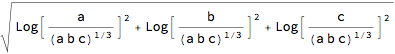
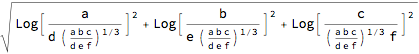
Graphs
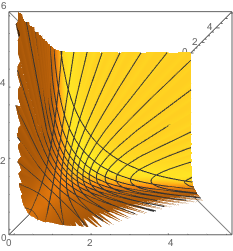
The following two graphs show the transformed data. We assume original co-ordinates that satisfy closure, with x + y + z = 1, and transform into new co-ordinates {x, y, z} / (x y z)^(1 / 3) and their logarithms.
Perhaps a 2D graph is just as clear but we want to relate to the unit simplex above.
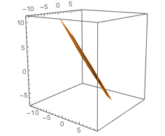
The first graph give the direct transform, the second graph gives the Log of this, and check that the latter is a plane (though Mathematica still draws contour lines because of minute numerical approximations).
ParametricPlot3D[z = 1 - x - y; If[z > 0, {x, y, z}/(x y z)^(1/3)], {x, 0, 1}, {y, 0, 1}, AspectRatio -> 1, ViewPoint -> Right]
ParametricPlot3D[z = 1 - x - y;
 If[z > 0, Log[{x, y, z}/(x y z)^(1/3)]], {x, 0, 1}, {y, 0, 1},
 AspectRatio -> 1, PlotRange -> All]
The triad of improduct, norm and distance
For the improduct, norm and distance it suffices to use the centered logratio transform. We do not have to assume closure.
?AitchisonImproduct

AitchisonImproduct[{a, b, c}, {d, e, f}]

AitchisonImproduct[seats2, votes2] // N
10.1515
As said, we do not have to assume that the vectors satisfy closure.
AitchisonImproduct[seats2, votes] // N
10.1515
?AitchisonNorm

AitchisonNorm[UnAit[]]
0
AitchisonNorm[{a, b, c}]
AitchisonNorm /@ {seats2, votes2} // N
{4.39063, 2.31295}
The Aitchison distance is the Euclidean distance for the rebased vectors.
If we do not use Norm but above AitchisonNorm then we divide instead of subtract, with the rationale that division for real data is subtraction for logarithms.
?AitchisonDistance

AitchisonDistance[{a, b, c}, {d, e, f}]
AitchisonDistance[{a, b, c}/ {d, e, f}, {1, 1, 1}]

AitchisonDistance[seats2, votes2] // N
2.07952
The outcome 2.1 differs quite a bit from the earlier finding of the Loosemore-Hanby outcome of 6%, yet, we have no standard to judge that value 2.1.
PM 1. In the theory of votes and seats, researchers already considered using the Log[seats / votes] transform. See Appendix D for its use in the Webster / Sainte-Laguë measure.
AitchisonDistance[seats2 / votes2, {1, 1, 1}] // N
2.07952
PM 2. Check again that it is not required to use closure data. (But for seats2 we flipped a seat.)
AitchisonDistance[seats2, votes] // N
2.07952
Underlying the Aitchison distance: Reportion and Stretch
For compositional data, Aitchision might have sufficed to argue that one should use the centered logratio transform, and then use the Euclidean improduct, norm and distance on those transformed vectors.
Instead, he also showed that this might be interpreted as a particular geometry on the unit simplex. The emphasis on "closure" and the unit simplex in the literature on the Aitchison distance only derives from this additional purpose. Since our present discussion aspires at a fair comparison of the methods, we now look at this additional purpose. Essentially, though, it is a distraction from the centered logratio transform.
Consider these two operations on the vectors in the unit simplex, which turn this into a vector space:
(1) Reportion, a.k.a. perturbation, which has the role of "addition" for the vector space.
(2) Stretch, a.k.a. power, which has the role of "scalar multiplication" for the vector space.
The routines assume that the input already is in closure.
Reportioning is when you have data in volumes and multiply these data with the densities to get data in weights.
?Reportion

Reportion[{a, b, c} , {d, e, f}]
Stretching is the application of a uniform power to all elements.
?Stretch

Stretch[{a, b, c}, p]
Stretch[{a, b, c}, -1]
For example, when x is on the unit simplex, with 1'x = 1, then (i) y = Sqrt[x]will be on the unit hypersphere, with || y || = 1, (ii) but Stretch[x, 1/2] will be on the unit simplex again.
nc = Norm[Sqrt[Closure[{a, b, c}]]] /. Abs -> Identity // Simplify
1
A vector space on the unit simplex with reportion and stretch
Reportioning and stretching generate a vector space for the variables under closure.
The Aitchison norm and distance satisfy the requirements for norm and distance, with the UnAit[] as the neutral element for addition. See the referred papers for the math. Appendix A shows this formally in Mathematica as well. For numbers it is more straightforward.
Reportion[votes2, Stretch[votes2, -1]] == UnAit[3]
True
For pairs x, there is the special property that the inverse operation Closure[x^(-1)] = 1 - x.
Stretch[{1/3, 2/3}, -1]
{2/3, 1/3}
Stretch[{x, 1 - x}, -1] // Simplify
{1 - x, x}
There seems to be a small tension between (a) the vector space under closure and (b) the use of Euclidean improduct, norm and distance for centered log-ratio vectors. However, the vector space under closure has its own definitions of improduct, norm and distance. Thus, when AitchisonNorm uses x / y in Euclidean terms, it actually uses Reportion[x, Stretch[y, -1]]] for the variables under closure, whence we have a theoretically closed system.
?AitchisonDistance

AitchisonDistance[seats2, votes2]
2.07952
AitchisonNorm[Reportion[seats2, Stretch[votes2, -1]]]
2.07952
Still a question on conceptual consistency
While we have consistency in terms of logic, this still leaves a question on conceptual consistency.
(i) For the Aitchison distance, the centered logratio transform is more important than closure, since this distance is invariant to scalar multiples per vector (and thus also to the scalars generated by the closure operation).
(ii) Applying closure afterwards to clr-transformed data generates zeros. Thus clr-data are not on the unit simplex.
(iii) Thus it is true that multiplication and power (Reportion and Stretch) generate a vector space on the unit simplex, but this is rather irrelevant for centered logratio data, which are not on that simplex. The clr-data are in Euclidean space and we can still use the Euclidean improduct, norm and distance (which generates the Aitchison distance for the original data).
Thus, my take on this part of the literature is:
(1) For compositional data for which the ratios are important, one would use the centered logratio transform, and then use the normal Euclidean improduct, norm and distance on those transformed data, including regressions and such (minding the loss of 1 degree of freedom). Forecasts can be interpreted again using Exp or the InverseCLR transformation.
?InverseCLR

(2) The invariance of the Aitchison distance to component-wise multiplication before the transform (e.g. changing volumes in weights) depends upon the properties of the clr-transform. Idem dito for scalar multiples and the power relationship. Closure is not relevant here but only the clr-transform. Empirical researchers would diagnose that clr-transforms are the proper data to work with. They would still discuss whether to use weights or volumes (sensitive to temperature) though, since these would generate different clr-transforms (though with the same distances).
(3) The Aitchison geometry, with the interpretation of multiplication and power as creating a geometry on the unit simplex, is a mathematical exercise that is not relevant for empirical researchers. There is a connection between (1) & (2) and (3), in that logarithms change multiplication into addition, but that is all. The mathematical content is not large either, and perhaps suitable for a first year course on normed spaces. The discussion about this geometry is distractive for empirical researchers, who do not deal with the unit simplex but with the clr-transforms. (For example, the creation of "lines" and "angles" on the unit simplex using this geometry is a mathematical exercise but conceptually at a distance for the clr-transforms that are not on the simplex.) It is true that one might interprete the camel as the "ship of the desert" but one should not be carried away by this interpretation.
(4) Thus the literature on "analysis on compositional data" can be cleaned up greatly but using these distinctions: (i) The explanation to empirical researchers on how to deal with compositional data that either satisfy the clr-transform (soil, milk) or not (votes and seats). (ii) A succinct text on that geometry for a first year course on normed spaces, not really relevant for researchers.
(5) I don't expect but am still open to the possibility that the geometry might generate surprise insights for research.
8. Aitchison geometry and voting data
Judging the application of the Aitchison geometry requires knowledge about the particular field of application. As an econometrician and researcher in didactics of mathematics, I cannot judge upon applications for issues of geology or biology and such. The use of the voting data fall under "political science of electoral systems" and this area overlaps with "political economy" and "public choice". See the reference to my paper on this.
We are looking for properties that are essential for our understanding of proportionality between votes and seats: (1) properties that apply to both the angular and Aitchison distance but for which the first is simpler, (2) properties that apply to the angular distance but not the Aitchison distance, (3) properties that apply to only the Aitchison distance and not the angular distance. (Potentially there is also: (4) properties that apply to neither.)
We already mentioned some drawbacks for the application of the Aitchison geometry to voting data: (1) the pairwise comparison of votes and seats, instead of having lots of samples on the same issue like for soil, (2) the essential zeros for parties who get votes and not seats, (3) the importance of the total available seats S for seats = Ap[votes, S], (4c) no adjustment of scales per party component.
Let us look further at (4c) Reportioning, (4d) subcompositional dominance.
Judging a distance by some reference
The Aitchison distance between the votes and seats of this basic example is, with an outcome close to 0:
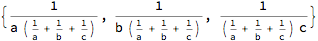
AitchisonDistance[{49, 51}, {51, 49}]

The Aitchison distance is invariant to reportioning:
AitchisonDistance[ {a, b} {49, 51}, {a, b} {51, 49}]

The Aitchison distance has a factor ?2. We might divide standardly by this, like we do for the Euclid / Gallagher index to correct for double counting of relocated seats.
We still lack a yardstick to interprete what remains. A point of reference is perhaps this case that we would consider to be close to a maximal difference (or find a House with more than 1000 seats):
AitchisonDistance[{999, 1}, {1, 999}]

Thus a relative distance might be:
AitchisonDistance[{49, 51}, {51, 49}]  /
  AitchisonDistance[{999, 1}, {1, 999}] // N
0.0057922
Section 4 already showed the transformation is d / (1 + d), though we must beware that it becomes rather insensitive at the extremes.
Reportioning of voting data 1: assuming perfection in apportionment
The question in this subsection is whether apportionment has the property Ap[x v, S] = x Ap[v, S] for arbitrary nonnegative vectors x.
We already have d[w, z] = d[w, Ap[w, S]]. Let us not assume just now that 1'(x w) = 1 too.
Above property gives d[x w, Ap[x w, S]] = d[x w, x Ap[w, S]] = d[x w, x z]. If apportionment causes an outcome d[w, z] then with above property apportionment also causes d[x w, x z] for any x. When this property would apply, then apportionment can be reduced to merely updating the seats with the change in votes.
In general, apportionment exists precisely since there is no such property that can be used like this. Perhaps for a rough estimate only.
If apportionment would be perfect then z = w, and d[w, z] = d[w, w] = 0. With this perfection, also d[x w, Ap[x w, S]] = 0. If above property would hold then d[x w, x z] = 0 too. Thus perfection and above property give d[w, z] = d[x w, x z] = 0 for any x. Unfortunately apportionment exists because there is no such perfection.
The following argues the same, now using explicitly two apportionments of seats given votes: s1 = Ap[v1, S] and s2 = Ap[v2, S].
When {v1, s1} would be the results of one election, and when a new election generates v2, then an estimate would be s1 * (v2 / v1) but we would rather await the process of apportionment as s2 = Ap[v2, S].
Define t = v2 / v1 and r = s2 / s1. We have s2 = Ap[t v1, S] and s2 = r s1 = r Ap[v1, S].
Thus Ap[t v1, S] = r Ap[v1, S]. Can we really assume that t ~ r ? In that case Ap[x v, S] = x Ap[v, S].
In practice we will have a relation that r = Ap[v t, S] / Ap[v, S] = r[v, t, S].
Suppose that we have a disproportionality measure such that disp[v1, s1] ~ 0 ~ disp[v2, s2].
Obviously disp[v2, s2] = disp[t v1, r s1] ~ disp[v1, s1], namely both close to zero.
Can this be seen as invariance of reportioning by t ~ r or v2 / v1 ~ s2 / s1 ?
If apportionment Ap is truely proportional, so that s1 / v1 = [Lambda] 1 and s2 / v2 = [Mu] 1, then r = s2 / s1 = ([Mu] v2) / ([Lambda] v1) = [Mu]/[Lambda] t. Thus r[v, t, S] = [Mu]/[Lambda] t, in which the complexity has been hidden in [Lambda] and [Mu]. Real numbers allow perfect apportionment, giving z = w, switching to unitised variables now. For perfection on these unitised variables, [Lambda] = [Mu] = 1. This is the case from above again, with d[w, z] = 0 and d[x w, x z] = 0, with the added restriction that 1'(x w) = 1. For seats we have rounding however. This rounding should perhaps not affect the choice of the distance measure. But rounding may still imply that we cannot rely upon an invariance to reportioning.
In practice there will be few cases such that t ~ r or v2 / v1 ~ s2 / s1, so that we may observe some invariance to reportioning.
It is more likely that there will be imperfections due to rounding. Invariance to reportioning would go against rounding.
The above assumes apportionment under a system of proportional representation. In district representation, the transformation of votes into seats is more complex, and there is no link to the supposed perfection of apportionment.
The comparison of votes and seats likely would do better by choosing an inequality / disproportionality measure that doesn't hinge upon invariance to reportioning.
The discussion whether such invariance Ap[x v, S] = x Ap[v, S] is relevant or practically possible distracts from the very purpose of apportionment.
Reportioning of voting data 2: differential growth of party sizes
For v1, v2, s1 and s2, let us suppose that Party A drops by about 40% of its votes and seats, and that Party B rises by about 40% of its votes and seats. These are only approximate effects, and we would get proper values from closure (and apportionment).
factor = {.6, 1.4}; {factor {4.9, 5.1}, factor {5.1, 4.9}}
{{2.94, 7.14}, {3.06, 6.86}}
In that case, the Aitchison distance remains the same. Let us use integers to generate the exact result.
factor = {6, 14}; {factor {49, 51}, factor {51, 49}}
{{294, 714}, {306, 686}}
factor = {6, 14}; AitchisonDistance[ factor {49, 51}, factor {51, 49}]

% // N
0.0565761
By comparison, the angular distance is slightly reduced from 0.25 grade to 0.18 grade, or from 2.5% to 1.8%, since the resulting vectors are closer together indeed.
factor = {6, 14}; AngularID[factor {49, 51}, factor {51, 49}] // N
0.184422
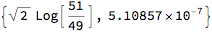
An extreme effect uses {1/1000, 1000}. The Aitchison distance does not change, as this depends upon the ratio Subscript[x, i] / Subscript[y, i] while the angular distance becomes close to zero because votes and seats get close to {0, 1}.
factor = {1/1000, 1000}; AitchisonDistance[ factor {49, 51}, factor {51, 49}]

factor = {1/1000, 1000}; AngularID[factor {49, 51}, factor {51, 49}] // N
5.10857*10^-7
PM. Closure has no effect on the outcome again, but can be shown anyway.
factor = {1/1000, 1000};
vts = Closure[factor {49, 51}] ;
sts = Closure[factor {51, 49}] ;
{vts, sts}

{AitchisonDistance[vts, sts], AngularID[vts, sts] // N}
In sum, the differential growth of party sizes suggests that invariance in reportioning is counterproductive.
Reportioning of voting data 3: policy distance
The next main section looks at policy distance, and contains a role for the AngularID[p v, p s], in which p are policy positions on a left-to-right scale [0, 10]. The measure used there cannot be based upon AitchisonDistance[p v, p s] since this is equal to AitchisonDistance[v, s].
Subcompositional dominance
For compositional data on minerals, a common dimension reduction is by dropping components in the vector, e.g. when the water content is removed, and the remainder components are rebased with "closure". There would be spurious correlation in the original data when columns on components are used instead of rows on samples.
An example in the literature
Martin-Fernandez et al. (undated, p2) contain an example on subcompositional dominance.
Consider (using "s" for "sub" and not "seats"):
x1 = {.1, .2, .7};
 s1 = Drop[x1, -1];
x2 = {.2, .1, .7};
 s2 = Drop[x2, -1];
Subcompositional dominance would require that dist[s1, s2] ? dist[x1, x2].
The formal definition is provided in Aitchison (undated) "Concise guide", p35.
Let us first look at the angular distances and then the Aitchison distance.
The angular distances are, using radians to link up with table 3 on p4 in Martin-Fernandez et al..
{VectorAngle[x1, x2] , VectorAngle[s1, s2],
 VectorAngle[Closure[s1], Closure[s2]]}
{0.192748, 0.643501, 0.643501}
For voting, these outcomes are logical. We should not confuse a comparison for three parties with a comparison for two parties. The participation of a third party may affect the evaluation of the total vectors of votes and seats.
(i) The x1 and x2 are closer together because the third party has been valued accurately. (ii) When we consider the situation with only two parties, then s1 and s2 are further apart, as votes {1/3, 2/3} have opposite seats {2/3, 1/3}. (iii) Thus, subcompositional dominance does not seem to be so useful for votes x1 and seats x2.
Degrees of freedom, dropping one element
This issue relates to the point that compositional data lose one degree of freedom. For the angular distance between votes and seats there is little reason to drop e.g. the last observation (potentially the essential zero) and then look at the angle between the remaining independent party shares. Namely, suppose that the last dependent share in each vector is the same, and that the other elements differ, like indeed is the case for above x1 and x2 and their subcompositions s1 and s2. Then the full vectors have a smaller angle, and we would want to see this reflected in the disproportionality measure (and thus we would not drop one element from the vector).
Ergo
Thus for voting we can properly infer that the situation with x1 and x2 with three parties is more proportional and that the situation with s1 and s2 with two parties is more disproportional.
The Aitchison distance however generates the same outcomes. The perfect match .7 for the third party is neglected, and the measure concentrates on where there are differences. We can also understand this outcome by reportioning as x1 / x2 = {1/2, 2, 1}, as another way to show that only the positions are used for which the ratios differ from 1.
{AitchisonDistance[x1, x2] ,
 AitchisonDistance[x1 / x2, {1, 1, 1}],
 AitchisonDistance[s1, s2],
 AitchisonDistance[Closure[s1], Closure[s2]]}
{0.980258, 0.980258, 0.980258, 0.980258}
Martin-Fernandez et al. (undated) conclude that the angular measure has no "compositional coherent behavior". If votes and seats are regarded as compositional data, then there is a distinction between votes and seats on the one hand and soil and milk on the other hand.
PM. A bit more about the application of the angular measure in geology
Martin-Fernandez et al. refer to a paper by Watson & Philip 1989 who propose the use of the angular measure for geological compositions. Unfortunately that paper is behind a paywall. Aichison, "Concise guide" p17 refers to this approach as being inappropriate for analysis of compositional data, referring to various other papers behind paywalls too.
Wang et. al 2007 project a vector of dimension n into a vector of dimension n - 1 consisting of angles between components, yet, this might be dependent upon permutation, as one would get different angles for different permutations.
See Appendix B for the relation between closure and the unit sphere.
9. Scoring parties on a policy scale
The parties can also be scored on a policy scale, say a vector p with elements in [0, 10]. A common term for such a scale is "left-to-right" even though those terms are rather out-dated. With unitised votes and seats w and z, a weighted average of the difference between House and electorate is a = p . (z - w). A basic reference is to Golder, M. & Stramski, J. (2010), "Ideological congruence and electoral institutions", American Journal of Political Science, 54(1), 90-106. For example, they state (p95): "(...) substantively representative legislatures [for us now: a = 0] increase things like perceived levels of democratic legitimacy and responsiveness, satisfaction with democracy, political participation, or personal efficacy and trust in the political process."
As a political economist, I regard it as "revealed preference" (a term coined by Paul Samuelson) what parties are voted for and what policies those parties enact. When researchers try to determine what the "policy stance" p of the parties is then this seems operationally dubious and needlessly complicated, since we already have the distinctions between parties with their votes and seats, including the angular distance d[v, s] between them. Remarkably, some researchers who prefer a policy distance tend to regard the distance between votes and seats as devoid of such meaning, and they thus do not value the interpretation in terms of revealed preference. The present discussion thus only occurs because there is a section in the literature that tries to look into such a policy distance between House and electorate.
The discussion on a policy distance measure has been split off as a separate paper, Colignatus (2018), since it distracts from the purpose of the present discussion, namely to compare with the Aitchison geometry.
In an earlier text (2017b, p45 and its Appendix J) I suggested that the angular distance d[p v, p s] might be a policy distance itself. I retract this suggestion. This is only true for the perspective of f[v, s ; p] = d[p v, p s] for a given p. There is a different perspective for g[p ; v, s] = d[p v, p s] for given w and z, which appears to be policy congruence and not incongruence. A widening policy gap between parties does not increase but reduce the angle of vectors p v and p s, since the components actually come closer to each other. We already saw this above for differential growth of party sizes. A clear example is using p = {0, 10} that causes an outcome of 0. Thus d[p v, p s] is a measure of disproportionality given p and a measure of congruence given v and s. This point has now be included in Colignatus (2018), while (2017b) needs an update.
Thus, Colignatus (2018) gives the revised suggestion for an angular policy distance pd[v, s, p] that uses a transform of angular d[p v, p s]. Such a proposal would not work for the Aitchison distance, in which dait[p v, p s] = dait[v, s] because of reportioning.
10. References in the voting literature to Aitchison's analysis
Votes and seats versus other purposes
The following papers don't discuss the distance between votes and seats, whence they were not referred to in the first versions of this paper. They refer to Aitchison and compositional data though, and it enhances completeness for the present discussion to mention these other papers after all
It remains important to distinguish between the different objectives of the analyses. While this present paper focuses on d[v, s] and Log[z / w], the following papers focus on v and Log[Subscript[w, i] / Subscript[w, j]] and their explanatory factors, like income and other social-economic factors. The following papers have regressions on v cq. its transform Log[w], whence they implicitly attach relevance to the distances between vote shares cq. their transforms. This does not necessarily imply that the distances between vote shares have the same meaning as the distances between votes and seats.
To deal with the summation (closure) condition, we could drop the party with the least reliable estimate of w and see whether the estimate improves by treating it as a remainder. The issue is whether the estimate or prediction improves by using logarithms. Since Log[x] ? x when x ? 1, the log transform may be superfluous for the bipartisan case with vote shares around 50% because of the median voter theorem.
In this subject matter on v and its explanatory factors, it is a cause of concern that not all parties participate in all districts. Observe that the use of w or even w / (1 - w) tends to be unproblematic when parties get 0 votes, while it would be exceptional when a party would get 100% of the vote: e.g. the exception of uncontested districts. An approach is to use dummies for whether a party participates or not, but there may also be combination effects, and one would not want that the dummies dominate the analysis. A recent suggestion for a general approach is by Blackwell, Honaker and King (2017).
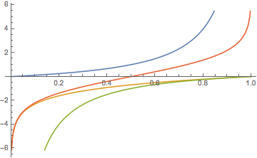
The following plot compares w / (1 - w) (blue) and Logw. Between 0.25 and 0.75 they are both fairly flat. Observe:
(1) If we use w / (1 - w) for values below 0.5 and Log[w] for values equal to or greater than 0.5 then we have a fairly flat transform, with the question why transform at all.
(2) If we use Log[w] for values below 0.5 and w / (1 - w) subsequently, then we have great dispersion. For Log[w] below 0.5 we might also use -(1-w)/w (green) of course. This kind of combination is actually achieved by Log[w/(1-w)], the logit transform (red).
The reason for a transform derives from an hypothesis on the error distribution, say the lognormal distribution. This is a specialist topic and a researcher would have to look into this before one can make comments on substance.
Plot[{w / (1 - w), Log[w], -(1 - w)/w, Log[w /(1 - w)]}, {w, 0, 1}]
Gelman & King 1994
Gelman & King (1994) consider the US bipartisan case. "We model district vote proportions directly, without the logit transformation used in King and Gelman (1991). The loss is very slight because contested district vote proportions above 0.8 or below 0.2 are rare." (p548). In uncontested districts, there are data problems, like zero votes, and the authors use imputation, for the counterfactual of what the vote might have been with a contest, with an algorithm that starts with 0.25 and 0.75 (their Appendix A). Perhaps a useful term is "model consistent imputation". The authors use the term "effective vote", but it is unclear what effectiveness would mean here, and it suffices to speak about "estimated vote".
Honaker, Katz & King (2002)
Honaker, Katz & King (2002) have a multiparty model and refer to compositional data and Aitchison. They apply the Log[v[i] / v[J]] transform a.k.a. the "additive log ratio" (ALR), i.e. divide by the vote share of the Jth party, and then consider only parties i = 1, ..., J - 1.
They explicitly do not follow Aitchison in the use of the lognormal function, and instead use the t distribution for the logs, and the logistic function at the level of the vote shares instead. However, this is no departure from the Aitchison geometry itself, that does not imply the use of the normal distribution.
They also apply (model consistent) imputations, for parties not participating in districts.
There is no implication that modeling Log[v / v[J]] in such manner would imply that votes and seats must be compared by Log[z / w] too. The authors use regression techniques that rely upon Euclidean space, with the Euclidean distance applied to these logratio transforms, and this implies the use of the Aitchison distance for the original shares w. But this need not imply that the apportionment of seats given the votes must be judged by the same distance measure.
Honaker & Linzer (2006)
Honaker & Linzer (2006) is a draft, and I have not been able to find a journal version.
The paper opens with the notion of compositional data. They mention that vote shares meet with more challenges than cases in the natural sciences: "because the categories of the composition may change between observations. First, within an election, not all parties may run on the ballot in all districts. Second, within a country, but across time, which parties exist may change, as may the total number of parties. Third, across countries the variety, platforms and number of parties certainly varies."
The authors concur that the coefficients of a model with ALR would be hard to interprete: "Each coefficient describes how the log ratio of some party changes with regards the reference party." The use of the ratio to the geometric mean (i.e. the centered logratio (CLR)) might give more stability. However, they refer to the bipartisan case as having a straightforward interpretation of the parameters, as the gain of one party is the loss of the other party. Also for more parties we may consider using Log[Subscript[w, i] / (1 - Subscript[w, i])] i.e. the logit-per-party, to get rid of a single reference party J. Given the binary (bipartisan) and centered cases, the logit-per-party cannot be excluded as unfit for the Aitchison framework. This framework essentially consists of using logarithms and dropping one variable to satisfy the summation (closure) condition. Dropping a variable removes a cause for dependent errors. Yet, for the distance between votes and seats we would not drop a party.
The authors usefully review the voting literature w.r.t. zero votes.
(1) Case by case modeling. For example use levels when votes are close to zero and 1, and logarithms elsewhere if the errors suggest a lognormal distribution. It would be better when this can by avoided by designing a general approach, see Blackwell et al. op. cit.
(2) Aitchison's suggestion was to impute a very small number, e.g. a trace element that is so small that it cannot be detected. For votes, there however are structural reasons for real zeros.
(3) Consider having a first stage that determines whether there is a zero or not, and a second stage dealing with non-zero's. This is a structured form of (1).
(4) The Katz & King (KK) approach of model-consistent imputation a.k.a. "effective vote". This is a form of (1) too.
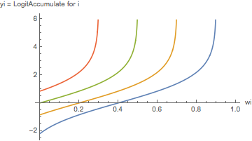
(5) The proposal by H&L themselves, to use a score on policy stances p, order the parties, and then consider the logit of the cumulated shares. Let W[j] = Subscript[?, i]^j w[i] then the transform would be y[i] = Log[W[i] / (1 - W[i])]. Ordering the parties will be simpler than pinpointing their exact positions.
?LogitAccumulate

LogitAccumulate[{.10, .15, .25, .50}]
{-2.19722, -1.09861, 0.}
LogitAccumulateInverse[%]
{0.1, 0.15, 0.25, 0.5}
The following continues with (5).
The cumulation will end in 1, so the last element(s) will be 1, and then the logit will be undefined, but this last party can be dropped. Parties with zero votes hopefully are not at the beginning or end. Their position should be determined by p. Parties with zero votes have the same cumulated scores as their previous parties. These same scores should be explained by different values of the explanatory variables.
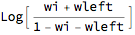
Let us see how a particular vote weight somewhere in the middle of a list relates to its transform. With w = {Subscript[w, 1], ..., Subscript[w, i], ...., Subscript[w, n]} the sum to the left can be represented by wleft and the sum to the right by 1 - wleft - Subscript[w, i]. We essentially have three "parties" and only need to select the 2nd element.
la[wleft_, wi_] = LogitAccumulate[{wleft, wi, 1 - wleft - wi}][[2]]
The following plots for different values of the sums to the left. Above we already got LogitAccumulate[.1] at -2.19722. The higher wleft, the sooner Subscript[w, i] starts rising dramatically. The linear approximation that works well for the bipartisan case around 50% has little relevance. When wleft = 0.1 then Subscript[w, i] still has a flat transform for about [0.2, 0.8]. But when wleft = 0.7 then Subscript[w, i] meets a steep curve.
Plot[Evaluate[la[#, wi] & /@ {.1, .3, .5, .7}], {wi, 0, 1},
 AxesLabel -> {"wi", "yi = LogitAccumulate for i"}]
The ordering goes against one of Aitchison's four criteria on the distance, namely permutation invariance (Section 5 above). For the distance between votes and seats this invariance is important. We must wonder whether such invariance would also be important for above y.
Conceptually, the y pertain to the social welfare function SWF of the voters. A SWF might say little about the shares w themselves. Thus the use of the transform y should not cause us to infer that H&L suggest another distance measure. Stated differently: finding a better estimate of w by use of a transform y does not imply that one discards common distance measures on w.
The logit of the bipartisan case clearly has its use, also with reference to a median voter on a policy scale p. The logit of the accumulated values merely extends this to various other positions on that scale. The logit of the accumulated values thus is an interesting transform but it is not clear a priory why it would generate better estimates.
While parties might compete with their policy neighbours, rather than with more distant parties, H&L explicitly provide for wider competition. This seems like an interesting consideration, but this tends to shift the discussion to policy position and policy distance, and, for us, away from distances in shares of votes or distances between votes and seats. The authors modify the cut-off points between parties in policy space with "valances", that seem to make the model rather complex and makes one wonder whether there still is a single policy space.
The logit of the accumulated values have a clear asymmetry. A party with a vote share of 0.2 meets linearity when wleft is small and meets with a stiff curve when wleft is large. Obviously, parties at the extremes have only one way to grow, towards the middle, while parties in the middle might grow in two directions. Thus the data have some asymmetry, but another one than this particular cumulation.
As a potential field of application the authors discuss the case that a party might consider not to partake in a ruling coalition out of fear of losing votes at a later election.
Multinomial probit and logit
Kropko (2008) does not refer to Aitchison but gives a useful comparison of multinomial probit and logit methods that puts above texts in perspective.
The logit approach assumes independence of the budget. The voter who must choose in a district between Conservatives, Labour or a Green Party would vote the same, regardless whether some party would participate in the district or not. The probit approach allows different vote shares depending upon the budget. Kropko relates this to what Kenneth Arrow called the "independence of irrelevant alternatives" (IIA). There definitely is a parallel between the mentioned budget dependence of voting shares and what Arrow discussed, but Arrow's topic is the construction of a social decision function or even ranking, and not just the establishment of voting shares. A better term for what Arrow intended is the "axiom of pairwise decision making" (APDM), since it allows that decisions are based upon pairwise comparisons. Colignatus (2001, 2014), "Voting theory for democracy", Chapter 9, discusses the meaning of this axiom for single seat elections. Thus it is fine that Kropko (2008) draws the parallel between the mentioned budget dependence and Arrow's analysis, but this IIA for voting scores and APDM for decisions should not be taken as identically the same. Taking them as the same is precisely the confusion between voting and deciding, which is a criticism w.r.t. Arrow's analysis.
11. Conclusion
Vectors of votes and seats, for (half) elections for political parties for say the House of Representatives, can be normalised to 1 or 10 / Ð or 100%, and then can be regarded as compositional data. The Aitchison geometry and distance for compositional data might also be applied to votes and seats. However, of seven criteria, votes and seats only satisfy two.
There is an essential zero when a party gets votes but doesn't gain seats. A zero gives an undefined logratio.
Votes and seats have a natural scale, namely the natural numbers, and the invariance to scale must only hold for the vectors as a whole: dividing the votes by turnout and dividing the seats by the number of seats in the House. The Aitchison distance is invariant to scale per component, so that e.g. volumes can be rescaled to weights. The latter property does not apply to votes and seats. One might argue that using the Aitchison distance for this case would not harm the analysis of the inequality / disproportionality of votes and seats. However, the issues of differential growth and the policy distance show that it does matter.
A key point is subcompositional dominance. For votes {1, 2, 7} and seats {2, 1, 7} it is essential that we consider three parties. For a distance or disproportionality measure we would value it positively that there is a match on 7. The Aitchison distance compares the ratio {1, 2, 7} / {2, 1, 7} = {1/2, 2, 1} with the ratio {2, 1, 7} /{2, 1, 7} = {1, 1, 1} and neglects a ratio equal to 1 since Log[0] = 1. It effectively compares the subcompositions, i.e. votes {1, 2} and seats {2, 1}, rescales to {1/3, 2/3} and {2/3, 1/3}, and finds high disproportionality. This means that it essentially looks at a two party outcome instead of a three party outcome.
Thus the comparison of votes and seats is an essentially different kind of analysis than for example the explanation of votes by means of political and social-economic variables. In the latter kind of analysis we would drop one variable to eliminate the dependence caused by the summation. In comparing votes and seats we would definitely not drop any variable, since the distance there would be relevant too, even when dependent upon the other variables.
It follows that votes and seats have a better measure in the angular distance (AID) and/or the Sine-Diagonal Inequality / Disproportionality (SDID) measure based upon this. One may of course use all measures, being aware of the crucial differences in meaning.
John Aitchison actually has two analyses. The literature would do well in making a clear distinction between: (1) the logratio transform and the Aitchison distance that are relevant for empirical research of compositional data, and (2) the Aitchison geometry on closure and the unit simplex that is mainly a mathematical exercise. Clearly the logratio transforms are not on the unit simplex.


