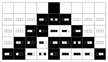
Here is an idea to display a CellularAutomaton evolution where every updated cell shows the neighborhood above it. This might be helpful when explaining to someone how it works.
ECAPlot[history_, opts___] :=
 With[{l = Length[history]},  Graphics[{EdgeForm[Gray],
    MapIndexed[{GrayLevel[1 - #], Rectangle[{#2[[2]] - 1, l - #2[[1]]}]} &, history, {2}],
    MapIndexed[Table[{GrayLevel[1 - #[[1, i]]],
        Rectangle[{#2[[2]] - 1 + .2 (i), l - #2[[1]] - 1 + .4}, {#2[[2]] - 1 + .2 (i + 1), l - #2[[1]] - 1 + .6}]}, {i, 3}] &,
     RotateRight /@ Most[Partition[history, {2, 3}, 1, 1]], {2}]}, opts]]
The update for each cell depends on the three cells above it, one to the left, one above and one to the right. The rule for the update stays the same. There are only eight cases for a rule so there are 256=2^8 rules. For more information see Wolfram's New Kind of Science. There are other ways for viewing rules like RulePlot but there should be more modern ways for helping explain how these simple rules work.
With the above code, the picture is from
ECAPlot[CellularAutomaton[30, {{1}, 0}, 4]]


