Throw

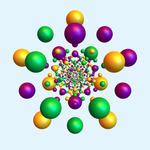
Once again, a Hamiltonian cycle on the vertices of a convex regular 4-polytope, stereographically projected to 3-dimensiona space. This time, it's the 120-cell, which has 600 vertices, which makes for a very long wait if you want to watch the entire cycle.

As usual, we need ProjectedSphere[], which stereographically projects a sphere inside the 3-sphere to 3-space; see Inside for the (long) definition of this function.

Now, inputting all 600 vertices is fairly annoying (Update: See @Ed Pegg’s reply below for a much cleaner solution). First of all, the vertices of the 24-cell are also vertices of the 120-cell:

twenty4cellvertices = 
  Normalize /@ 
   DeleteDuplicates[
    Flatten[Permutations /@ ({-1, -1, 0, 0}^Join[#, {1, 1}] & /@ Tuples[{0, 1}, 2]), 1]];

Aside from that, there are six other classes of vertices (this was cribbed from the Wikipedia entry a couple of years ago, and could definitely be re-written in a nicer way):

one20cellvertices1 =
  DeleteDuplicates[
   Flatten[
    Permutations /@ ({1, 1, 1, Sqrt[5]}*{-1, -1, -1, -1}^# & /@ 
       Tuples[{0, 1}, 4]), 1]];
one20cellvertices2 =
  DeleteDuplicates[
   Flatten[
    Permutations /@ ({GoldenRatio^(-2), GoldenRatio, GoldenRatio, 
          GoldenRatio}*{-1, -1, -1, -1}^# & /@ Tuples[{0, 1}, 4]), 1]];
one20cellvertices3 =
  DeleteDuplicates[
   Flatten[
    Permutations /@ ({GoldenRatio^(-1), GoldenRatio^(-1), 
          GoldenRatio^(-1), GoldenRatio^2}*{-1, -1, -1, -1}^# & /@ 
       Tuples[{0, 1}, 4]), 1]];
one20cellvertices4 =
  DeleteDuplicates[
   Flatten[
    Outer[
     Permute, ({0, GoldenRatio^(-2), 1, GoldenRatio^2}*{-1, -1, -1, -1}^# & /@ Tuples[{0, 1}, 4]), 
     GroupElements[AlternatingGroup[4]], 1], 1]];
one20cellvertices5 =
  DeleteDuplicates[
   Flatten[
    Outer[
     Permute, ({0, GoldenRatio^(-1), GoldenRatio, Sqrt[5]}*{-1, -1, -1, -1}^# & /@ Tuples[{0, 1}, 4]), 
     GroupElements[AlternatingGroup[4]], 1], 1]];
one20cellvertices6 =
  Flatten[
   Outer[Permute, ({GoldenRatio^(-1), 1, GoldenRatio, 2}*{-1, -1, -1, -1}^# & /@ Tuples[{0, 1}, 4]), 
    GroupElements[AlternatingGroup[4]], 1], 1];

And so we combine them all into one long list:

one20cellvertices = 
  Join[2 Sqrt[2] twenty4cellvertices, one20cellvertices1, 
   one20cellvertices2, one20cellvertices3, one20cellvertices4, 
   one20cellvertices5, one20cellvertices6];

Now, as in the case of Touch ’Em All and All Day, the idea is to use FindHamiltonianCycle[] to find a Hamiltonian cycle. Unfortunately, if you just plug in the one20cellvertices without modification, this will just run for hours and never terminate. However, randomly permuting one20cellvertices and then running FindHamiltonianCycle[] seems to almost always work. Here's the code (of course, if you evaluate this, you will get a your own unique cycle, almost certainly different from the one shown in the animation):

sorted120CellVertices = 
  Module[{v = RandomSample[one20cellvertices], M, g, 
    cycle},
   M = ParallelTable[
     If[N[EuclideanDistance[v[[i]], v[[j]]]] == N[3 - Sqrt[5]], 1, 0],
     {i, 1, Length[v]}, {j, 1, Length[v]}];
   g = AdjacencyGraph[M];
   cycle = FindHamiltonianCycle[g];
   v[[#[[1]] & /@ (cycle[[1]] /. UndirectedEdge -> List)]]
   ];

Next, I wanted the motion to be not quite linear, but much closer to linear than what you get by applying Smoothstep or one of its variants. Of course, $\text{Smoothstep}(t) = a + bt + ct^2 + dt^2$, where the parameters $a,b,c,d$ are given by

Block[{f},
 f[t_] := a + b t + c t^2 + d t^3;
 Solve[f[0] == 0 && f[1] == 1 && f'[0] == 0 && f[1/2] == 1/2, {a, b, c, d}]
 ]

So for a less smooth function I just used the parameters which solve the similar system

Block[{f},
 f[t_] := a + b t + c t^2 + d t^3;
 Solve[f[0] == 0 && f[1] == 1 && f'[0] == 2/3 && f[1/2] == 1/2, {a, b, c, d}]
 ]

This gives my function unsmoothstep[]:

unsmoothstep[t_] := (2 t)/3 + t^2 - (2 t^3)/3;

Finally, then, we can put it all together (notice that Lighting is just the standard lighting, but with ambient light which isn't so dark):

DynamicModule[{n = 3, θ, viewpoint = 1/2 {-1, 1, 1},
  pts = N[Normalize /@ sorted120CellVertices],
  cols = RGBColor /@ {"#06BC40", "#F8B619", "#880085", "#E4F4FD"}}, 
 Manipulate[θ = 
   ArcCos[1/8 (1 + 3 Sqrt[5])] unsmoothstep[Mod[t, 1]];
  Graphics3D[
   {Specularity[.8, 30],
    Table[
     {cols[[Mod[i - Floor[t], n, 1]]],
      ProjectedSphere[
       RotationMatrix[θ, {pts[[i]], pts[[Mod[i + 1, Length[pts], 1]]]}].pts[[i]], .06]},
     {i, 1, Length[pts]}]},
   ViewPoint -> {Sin[(
      ArcCos[Sqrt[1/6 (3 - Sqrt[5])]] ArcCos[
        2 Sqrt[6/(27 + Sqrt[5])]])/
      ArcCos[Root[841 - 3512 #1^2 + 2896 #1^4 &, 3]]], 0, 
     Cos[(ArcCos[Sqrt[1/6 (3 - Sqrt[5])]] ArcCos[
        2 Sqrt[6/(27 + Sqrt[5])]])/
      ArcCos[Root[841 - 3512 #1^2 + 2896 #1^4 &, 3]]]},
   ViewVertical -> {1, 0, 0}, PlotRange -> 10, 
   SphericalRegion -> True, ViewAngle -> 2 Pi/9, Boxed -> False, 
   Background -> cols[[-1]], ImageSize -> 500,
   Lighting -> {{"Ambient", RGBColor[0.52, 0.36, 0.36]},
     {"Directional", RGBColor[0, 0.18, 0.5], ImageScaled[{2, 0, 2}]},
     {"Directional", RGBColor[0.18, 0.5, 0.18], ImageScaled[{2, 2, 3}]},
     {"Directional", RGBColor[0.5, 0.18, 0], ImageScaled[{0, 2, 2}]},
     {"Directional", RGBColor[0, 0, 0.18], ImageScaled[{0, 0, 2}]}}],
  {t, 0, n}]
 ]

The coefficient of unsmoothstep[t] in the definition of θ is just the angle between adjacent vertices of the 120-cell.

It's easy to use a different number of colors by adjusting n to be another divisor of 600 (and of course by adding more colors to cols).