We discuss the changes to the interest rates processes when we move from mono-curve setting to multi-curve framework. This is characterised by presence of several curves a dedicated discount curve and set of estimation curves each for specific Libor rate. The first is generally assumed to be the OIS curve, whilst the rest are tenor curves for given Libor tenor.
The changes in the forward Libor estimation are due to the loss of martingale property when mono-curve world is replaced by multiple curve framework. We show how multiplicative adjustment works in this new setting and how interest rate derivatives are affected. Various modelling assumptions are used to show derivatives pricing in this new setting.
Introduction
We review the setting of Interest rate derivatives in post-crisis era characterised by multi-curve environment where dedicated yield curves are defined for forward rate estimation and cashflow discounting. The multi-curve framework is a direct consequence of financial crisis of 2007-2008 when the so-called 'Libor market' - represented by single yield curve stopped being seen as risk-free, and new curves started to emerge to better reflect the counterparty risk in the financial markets.
The current interest rate framework exists in the simplest form in the dual curve setting - (i) discounting curve - usually built with OIS instruments and (ii) estimation curve - generally used to build the 'main' estimation curve in a given currency. This is 3 month Libor curve for USD or 6 months Euribor curve for EUR.
Existence of dual curve environment does change the interest rate mathematics. Martingales defined in the single curve framework do not hold and the process has to be adapted to account for curves duality. We demonstrate how this process work and show how interest rate derivatives - both linear and optional work when we move from the singe to dual framework.
Interest rate derivatives in a single curve framework
We firs look at the single-curve homework in the pre-2007 era. When only one yield curve exists, the derivatives pricing is simple and tidy. Forward rate defined on the singe curve using two deposits coincides the forward rate agreement rate = FRA rate
Subscript[F, S] = 1/(Subscript[T, 2] - Subscript[T, 1]) * P[0, Subscript[T, 1]]/P[0, Subscript[T, 2]] - 1;
where Subscript[F, S] is the forward rate in a single-curve setting, Subscript[T, 1], Subscript[T, 2] and tow maturity dates with Subscript[T, 2]>Subscript[T, 1] and P[0, Subscript[T, 1]] , P[0,Subscript[T, 2]] are two discount factors at time 0 with maturities Subscript[T, 1] and Subscript[T, 2]. The FRA rate is then defined as Subscript[F, FRA] = K such that the payoff of the contract at time 0 has value = 0 L[Subscript[T, 1], Subscript[T, 2]] - K = 0 with L[Subscript[T, 1], Subscript[T, 2]] defined as forward term-rate.
Interest rate swaps in single-curve setting
Interest rate swap together with FRA are one the simplest linear interest rate derivatives. It usually involves exchange of fixed rate for a series of floating forward rates up to final maturity:
fixedLeg = S Sum[\[Delta][i] P[0, i], {i, 1, m}]
floatLeg = Sum[\[Delta][i] P[0, i] Subscript[L, S][i], {i, 1, n}]
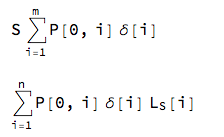
where $L_S$ is the forward Libor rate in a single curve framework. This is identical to the FRA rate defined above:
Subscript[L, S][i] = 1/\[Delta][i]*(P[i - 1]/P[i]-1)

floatLeg =
 Sum[\[Delta][i]*
   P[0, i]*(1/\[Delta][i])*(P[0, i - 1]/P[0, i] - 1), {i, 1, n}]
P[0, 0] - P[0, n]
Then swap rate S is simply a solution to the equation:
Solve[fixedLeg == floatLeg, S]
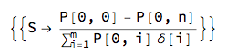
This shows that in a single-curve framework the swap rate is simply a difference in two discount factors normalised by $annuity= \sum_{i = 1}^n\delta[i]\ P[0, i]$. The same curve is used to produce discount factors that are used for (i) discounting and (ii) forward Libor estimation.
Multi-curve framework for Interest rate derivatives
When we move to multi-curve setting, we assume:
- Separate discounting curve - generally OIS curve
- Separate estimation curve for 'main index - 3M or 6M
- Separate estimation curves for 'minor indices - say 1M, 12M or 6M (in 3M setting)
When the discounting curve is set to the OIS curve, we define the OIS forward rate with tenor h similarly to the forward in the mono-currency setting: 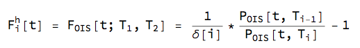
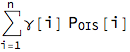
for i = 1...n where $\delta[i]$ is a year fraction for interval $T_{i-1} -T_i$ and $P_{OIS}[t,T_i]$ is a discount factor from the OIS curve at time t maturing at time $T_i$
In the multi-curve framework, the Libor definition in the single curve environment does not hold L[Subscript[T, 1],Subscript[T, 2]]] != Subscript[F, S][t;Subscript[T, 1],Subscript[T, 2]] != Subscript[F, OIS][t,Subscript[T, 1],Subscript[T, 2]] since the discount factors in definition of Libor when only one curve is used is not the same as in dual curve case. Libor is dual curve setting is calculated from the estimation curve with unique set of discount factors.
The expectation of forward Libor in the dual curve setting can be expressed as \!( *SubsuperscriptBox[(E), (t), SubsuperscriptBox[(Q), (OIS), (T2)]]([))Subscript[F, D][Subscript[T, 1];Subscript[T, 1],Subscript[T, 2]]] = Subsuperscript[E, t, Subsuperscript[Q, OIS, T2]][E^Subsuperscript[Q, OIS, T2][L[Subscript[T, 1],Subscript[T, 2]|Subscript[[ScriptCapitalF], t]]. The valuation of forward rate agreement with Libor forward rate is therefore defined as: FRA[t,Subscript[T, 1],Subscript[T, 2]] =Subscript[P, OIS][t,Subscript[T, 2]] [Delta][Subscript[T, 1],Subscript[T, 2]] \!( *SubsuperscriptBox[(E), (t), SubscriptBox[(Q), (OIS)]]([))L[t,Subscript[T, 1],Subscript[T, 2]]-K].
Current market practice takes a shortcut and simply values the FRA as FRA[t,Subscript[T, 1],Subscript[T, 2]] =Subscript[P, OIS][t,Subscript[T, 2]] [Delta][Subscript[T, 1],Subscript[T, 2]] (L[t,Subscript[T, 1],Subscript[T, 2]]-K]) where discount factor Subscript[P, OIS][t,Subscript[T, 2]] comes from the OIS curve and the forward Libor L[t,Subscript[T, 1],Subscript[T, 2]] is taken from the estimation curve. This is clearly inconsistent since forward Libor is NOT martingale under the OIS forward measure.
Libor adjustment in multi-curve framework
To restore the non-arbitrage relationship, forward Libor rate has to be adjusted. We refer to this as Forward basis that restores the equilibrium between Subscript[F, OIS] and Subscript[F, E]. Assuming multiplicative basis Aj, we get:
Fd = (1/\[Delta]) (Pd[T1]/Pd[T2] - 1);
Fe = (1/\[Gamma]) (Pe[T1]/Pe[T2] - 1);
Solve[Fe \[Gamma] == Fd \[Delta] Aj, Aj]
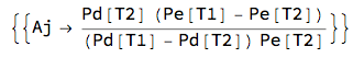
where Subscript[F, d] represents forward rate from the OIS curve, Subscript[F, e] is the forward Libor from the estimation curve, Subscript[P, d] is a discount factor f from the OIS curve and Subscript[P, e] is a discount factor from the estimation curve.
The forward basis is therefore a ratio of discount factors from both curves and can be recovered ex-post once both curve have been calibrated to the market data.
From modelling perspective, however it is desirable to express the forward rate in terms of single curve. We introduce new discount factor adjustment Subscript[B, j] and re-calculate the forward adjustment spread:
Fd = (1/\[Delta]) (PdT1/PdT2 - 1);
Fe = (1/\[Gamma]) (PeT1/PeT2 - 1);
PeT1 = BjT1 PdT1;
PeT2 = BjT2 PdT2;
Solve[Fd == Fe Aj, Aj] // Simplify
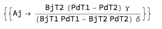
and get the forward Libor $F_e$
Fe
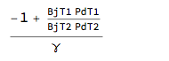
This shows that the Libor is a function of (i) OIS curve and (ii) discount factor adjuster. To proceed, we assume that the forward rate follows LogNormal martingale dynamics under forward measure Subscript[Q, e]
Fe = GeometricBrownianMotionProcess[0, \[Sigma], x0];
Fe[t]

![enter image description here][8]
We apply to similar process to the forward adjuster defined under forward measure $Q_d$
Bj = GeometricBrownianMotionProcess[0, \[Eta], y0];
Bj[t]
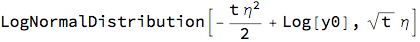
To change the measure from Subscript[Q, e]==> Subscript[Q, d], we use the change-of-measure technique that says:
Subscript[E, OIS][Fe] = Subscript[E, e][Fd Bj]. To change the measure, we need joint expectation of OIS forward and the forward adjuster. We apply the Binormal Copula with LogNormal marginals
cDist = CopulaDistribution[{"Binormal", ?}, {Fe[t], Bj[t]}];
cdrift = Expectation[x*y, {x, y} \[Distributed] cDist,
  Assumptions ->
   t > 0 && ? > 0 && ? > 0 && -1 <= ? <= 1]

The joint expectation of forward OIS and forward adjuster on relative basis provides the adjustment for the process where the change of measure occurs. Since the martingale process for forward Libor has to be drift less, we adjust the forward rate by its negative quantity;
Aj = cdrift/(x0 y0) /. t -> -t

Returning back to our original Libor adjustment formula, we observe: 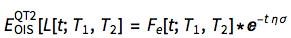
Fe_Adj = Expectation[x, x \[Distributed] Fe[t],
    Assumptions -> t > 0 && ? > 0 && x0 > 0]*Aj /. x0 -> L[0]

This is the forward Libor rate under the OIS forward discounting measure. The adjustment is a function (i) time, (ii) volatility of Libor and (iii) volatility of OIS rate. A reader familiar with the exposition above, an recognise here the parallelism to process drift adjustment in the foreign currency market know as 'quanto adjustment'. The similarity is obvious - we work with two curves, two sources and randomness and switch the measure similarly to what we do in foreign currency markets.
Forward rate agreement - FRA
This is the simple contract that pays the difference between forward Libor and fixed rate 
where [DoubleStruckCapitalC] is nominal and $\delta[\tau]$ is a year fraction on day count convention between the Libor tenor $T_1$ and $T_2$.
Ho much does the adjustment affects the FRA valuation? We look first at market volatilities - (i) for the Libor rate and (ii) Adjuster:
Assume: $\delta=0.25$, C=1 mil, $P_{OIS}[t,T_2] = 0.98$, t=1, L=0.0125,K=0.0125
fra = C*Pois*?*(L*E^(-t*?*?*?) - K) /. {C ->
    1000000, L -> 0.0125, K -> 0.0125, t -> 1, ? -> 0.25,
   Pois -> 0.98, ? -> 0.75}
Plot3D[fra, {?, 0.1, 0.3}, {?, 0.1, 0.3},
 AxesLabel -> Automatic, PlotTheme -> "Marketing",
 PlotLabel ->
  Style["FRA valuation impact by market volatilities", Blue, 15]]

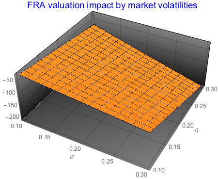
As we can see from the graph above, higher volatilities will push the value of forward rate lower and therefore making the value of long forward contract more negative. The opposite applies to a short FRA contract.
We can now look at correlation impact:
fra2 = C*Pois*?*(L*E^(-t*?*?*?) - K) /. {C ->
     1000000, L -> 0.0125, K -> 0.0125, t -> 1, ? -> 0.25,
    Pois -> 0.98, ? -> 0.2, ? -> 0.2};
Plot[fra2, {?, -0.75, 0.75}, PlotStyle -> Red,
 PlotLabel -> Style["Correlation impact on FRA valuation", Blue, 15]]
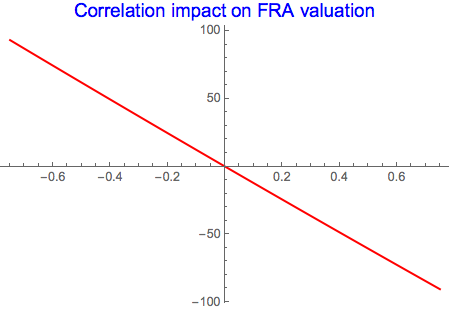
Negative correlation will increase the long FRA value since the adjusted Libor will be higher. Positive correlation will drive the valuation i into negative territory.
Interest rate swap - IRS
The payer IRS formula is determined from the same equation: fixed leg = float leg
fixedLeg = K Sum[?[i] Subscript[P, OIS][i], {i, 1, m}];
floatLeg =
  Sum[?[i] Subscript[P, OIS][i] L[
     i] Exp[-Subscript[t, i] ? ? ?], {i, 1, n}];
swapR = Solve[fixedLeg == floatLeg, K] // Simplify
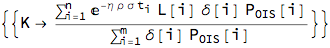
This is the equilibrium swap rate that will make present value at inception zero. The new formula differs from the swap rate formula in the single curve framework in two instances:
- Discount factor P comes from a special discounting curve - the OIS curve and becomes Subscript[P, OIS][t,Subscript[T, i]]
- Numerator does not reduce to a simple difference of two discount factors since adjusted Libor rate L[t, Subscript[T, 1],Subscript[T, 2]] E^(-t [Rho] [Eta] [Sigma]) is now estimated on a different curve, the so-called estimation curve
Caps and Floors
Consider first a Caplet paying out at time Subscript[T, k]. Caplet is essentially a call option on forward Libor rate L[t;Subscript[T, k-1],Subscript[T, k]]: [Delta][[Tau]] *(L[t;Subscript[T, k-1],Subscript[T, k]]-K)^+ where [Delta][[Tau]] is a year fraction between Subscript[T, 1] and Subscript[T, 2] and K is a fixed strike rate. The pricing formula is simply a discounted conditioned expectation of the payoff positivity under certain distributional assumptions. So, to price a Caplet in multi-curve framework, we proceed as in mono-currency case, with replacement: Libor mono-curve -> Libor multi-curve: 
Pricing formula will differ depending on the choice distributional assumptions for the forward Libor rate. For calculation purposes, we set the adjusted Libor rate -Subscript[L, e][t;Subscript[T, 1],Subscript[T, 2]] E^(-t [Rho] [Eta] [Sigma]) = x0. We choose the three processes that become the most common in the market - i.e. (i) Normal process, (ii) LogNormal process and (iii) Mean-reverting Normal process.
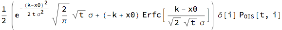
Normal process:
nProc = OrnsteinUhlenbeckProcess[0, ?, 0, x0];
nCplt = Subscript[P, OIS][t, i] ?[i] Expectation[Max[x - k, 0],
     x \[Distributed] nProc[t],
    Assumptions -> ? > 0 && t > 0] // FullSimplify
We can now investigate the behaviour of the Caplet w..r.t Libor volatility and strike
Plot3D[nCplt /. {Subscript[P, OIS][t, i] -> 0.98, ?[i] -> 0.25,
    x0 -> 0.0125, t -> 1}, {?, 0.005, 0.015}, {k, 0.01,
  0.0135}, PlotLabel ->
  Style["Caplet Normal premium", Blue, {15, Bold}],
 PlotLegends -> Automatic, AxesLabel -> Automatic,
 ColorFunction -> "Rainbow"]
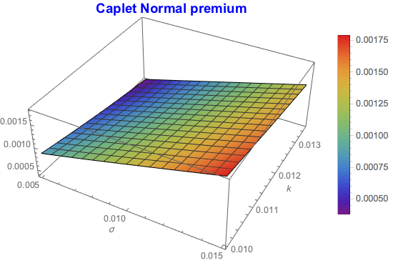
Premium increases as volatility goes up and strike declines. However, volatility is more dominant factor.
Lognormal process
lProc = GeometricBrownianMotionProcess[0, ?, x0];
lCplt = Subscript[P, OIS][t, i] ?[i] Expectation[Max[x - k, 0],
     x \[Distributed] lProc[t],
    Assumptions -> ? > 0 && t > 0 && k > 0 && x0 > 0] //
  FullSimplify

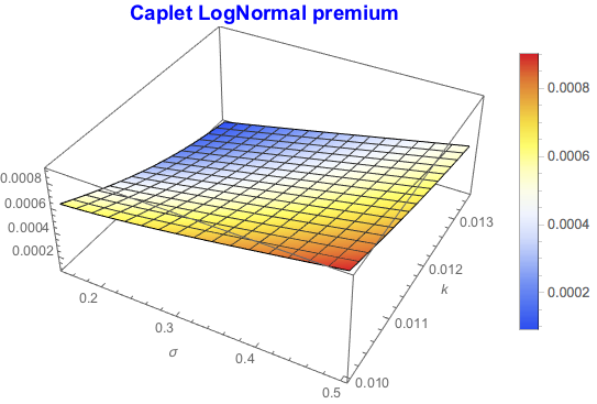
A similar pattern is observed for other processes, such as LogNormal
Plot3D[lCplt /. {Subscript[P, OIS][t, i] -> 0.98, ?[i] -> 0.25,
    x0 -> 0.0125, t -> 1}, {?, 0.15, 0.5}, {k, 0.01, 0.0135},
 PlotLabel -> Style["Caplet LogNormal premium", Blue, {15, Bold}],
 PlotLegends -> Automatic, AxesLabel -> Automatic,
 ColorFunction -> "TemperatureMap"]
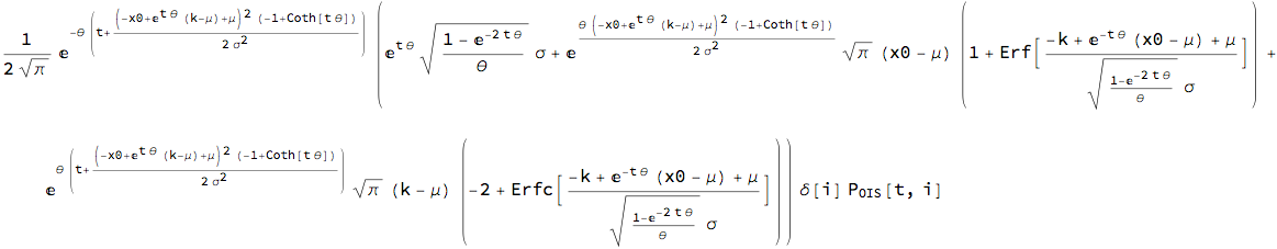
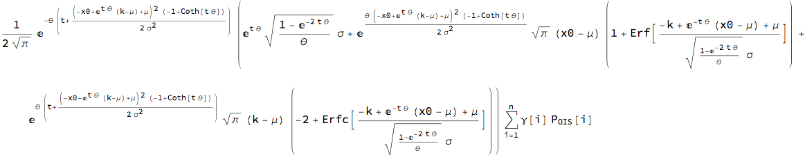
Mean-reverting normal process
mProc = OrnsteinUhlenbeckProcess[?, ?, ?, x0];
mCplt = Subscript[P, OIS][t, i] ?[i] Expectation[Max[x - k, 0],
     x \[Distributed] NormalDistribution[a, b],
    Assumptions -> b > 0 && t > 0];
mCplt = % /. {a -> mProc[t][[1]], b -> mProc[t][[2]]} // FullSimplify
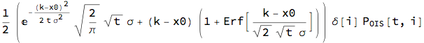
Floors
Interest rate floors are are essentially put options on forward Libor rate with payoff function:

Normal process
nProc = OrnsteinUhlenbeckProcess[0, ?, 0, x0];
nFlrt = Subscript[P, OIS][t, i] ?[i] Expectation[Max[k - x, 0],
     x \[Distributed] nProc[t],
    Assumptions -> ? > 0 && t > 0] // FullSimplify
LogNormal process
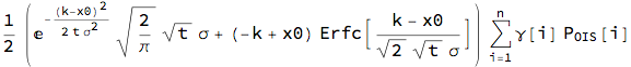
lFlrt = Subscript[P, OIS][t, i] ?[i] Expectation[Max[k - x, 0],
     x \[Distributed] lProc[t],
    Assumptions -> ? > 0 && t > 0 && k > 0 && x0 > 0] //
  FullSimplify

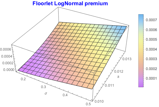
Plot3D[lFlrt /. {Subscript[P, OIS][t, i] -> 0.98, ?[i] -> 0.25,
    x0 -> 0.0125, t -> 1}, {?, 0.15, 0.5}, {k, 0.01, 0.0135},
 PlotLabel -> Style["Floorlet LogNormal premium", Blue, {15, Bold}],
 PlotLegends -> Automatic, AxesLabel -> Automatic,
 ColorFunction -> "Pastel"]
Swaptions
Swaptions are options on the swap rate defined above. They exist in tow formats: (i) Payer swaption = put option on the swap rate and (ii) Receiver swaption = call option on the swap rate. When we operate in the multi-curve framework, we deal with the same problem as in Libor case - i.e. swap rate adjustment.
We develop the swap adjustment in the same way as Libor. When LogNormal dynamics for the swap rate is envisaged, we arrive at the adjustment quantity though a joint expectation process:

The volatilities in the exponent are now swaption volatilities and correlation coefficient $\rho$ is the correlation between the swap rate and the adjuster.
Receiver swaption
This is the call option on the swap rate with the payoff ; Rec_OSWP = Subscript[AF, OIS] (Subscript[S, ADJ][t; Subscript[T, 0],Subscript[T, n]] -K)^+ where:
Subscript[AF, OIS] = Sum[?[i] Subscript[P, OIS][i], {i, 1, n}]
The option premium will depend on the modelling choice for the underlying swap rate. We look again at (i) Normal process, (ii) LogNormal process and (iii) Mean-reverting Normal process:
Normal process
nSwpn = Subscript[AF, OIS]
    Expectation[Max[x - k, 0], x \[Distributed] nProc[t],
    Assumptions -> ? > 0 && t > 0] // FullSimplify
LogNormal process
lSwpn = Subscript[AF, OIS]
    Expectation[Max[x - k, 0], x \[Distributed] lProc[t],
    Assumptions -> ? > 0 && t > 0 && k > 0 && x0 > 0] //
  FullSimplify

Normal mean-reverting process
mCplt = Subscript[AF, OIS]
    Expectation[Max[x - k, 0],
    x \[Distributed] NormalDistribution[a, b],
    Assumptions -> b > 0 && t > 0];
mCplt = % /. {a -> mProc[t][[1]], b -> mProc[t][[2]]} // FullSimplify
Payer swaption
These are put opinions on the swap rate which in case of multi-curve environment is drift-adjusted. For example, if we assume normal distribution for the swap rate, we get
Normal process
nSwpn2 = Subscript[AF, OIS]
    Expectation[Max[k - x, 0], x \[Distributed] nProc[t],
    Assumptions -> ? > 0 && t > 0] // FullSimplify
Conclusion
Multi-curve framework in case of interest rate derivatives brings new paradigm that requires certain adjustment to the underlying rates. This is due to a measure change when the expectation of the rates stops being martingale. Introduction of separate discounting curve - OIS requires adjustment to the forward rate drift in order to preserve non-arbitrage condition. Quarto-style adjustment known in foreign currency market is being used to derive neat formula.
Pricing and valuation adjustment with Mathematica, as the above demonstration shows, is easy. Availability of stochastic routines and probabilistic functions leads to quick and elegant solution.


