I tried it a bit different with a somewhat disturbing result

the undefined inner integral

j0 = \[Integral](Sqrt[196 - y^2 - x^2]) \[DifferentialD]x

insert the the upper bound yields a division by zero

j12 = j0 /. x -> Sqrt[14^2 - y^2] // Simplify

So try a limit, which seems to work

j12 = Limit[j0 /. x -> u, u -> Sqrt[14^2 - y^2]]

The lower limit is no problem

j11 = j0 /. x -> a + y/e

so the resulting inner integral should be

j2 = j12 - j11

Specify that for a = 1 and e = 1

j211 = j2 /. a -> 1 /. e -> 1

The upper bound for the outer integral is (and directly specified for a = e = 1 )

uL = (-a e + e Sqrt[196 + 196 e^2 - a^2 e^2])/(1 + e^2);
uL11 = uL /. {a -> 1, e -> 1}

But the integration gives something different from f [ 1, 1 ] given above:

In[11]:= NIntegrate[j211, {y, 0, uL11}]

Out[11]= -1843.8

Where is the flaw?

I think that is not true, especially when taking into account that Sqrt[ 196 -x^2- y^2 ] is not a complex function. The flaw is the strict confidence in the Limit Procedure, which gave

1/4 \[Pi] (-196 + y^2)

as value of the inner integral at the upper bound. When I had a close look at this limit

Limit[j0 /. x -> uu Sqrt[14^2 - y^2], uu -> 1]

it turned out that the negative value must be used. So writing

j2 = -j12 - j11 // FullSimplify

instead of the j2 given above and

jj2[a_, e_, y_] := Evaluate[j2]

and

ff[a_, e_] :=  NIntegrate[   jj2[a, e, y], {y,  0, ((-a)*e + e*Sqrt[196 + 196*e^2 - a^2*e^2])/(1 + e^2)}]

which when plotting gives the same picture as the other pics above

Plot3D[ff[a, e], {a, 0.01, 2}, {e, 0.01, 2}, ColorFunction -> "SolarColors"]

What is the learning? Mathematica is really a great software, but you can't always believe everything.

The flaw was that I didn't check if this limiting process gave a correct answer.

Adding assumptions seems to help. Below is one possibility. It took many minutes to evaluate though.

In[1]:= Integrate[Sqrt[196 - x^2 - 
       y^2], {y, 0, 
     ((-a)*e + e*Sqrt[196 + 
                196*e^2 - a^2*e^2])/
       (1 + e^2)}, {x, a + y/e, 
     Sqrt[14^2 - y^2]}, Assumptions -> {0 < a < 14, e > 0}]

(* Out[1]= ConditionalExpression[(1/(
 12 (1 + e^2)^(
  3/2)))(2 a^2 e Sqrt[(196 - a^2) (1 + e^2)] - 588 a e \[Pi] - 
   588 a e^3 \[Pi] + a^3 e^3 \[Pi] - 5488 Sqrt[1 + e^2] \[Pi] - 
   5488 e^2 Sqrt[1 + e^2] \[Pi] + 5488 I Sqrt[1 + e^2] Log[2] + 
   5488 I e^2 Sqrt[1 + e^2] Log[2] - 2744 I Sqrt[1 + e^2] Log[3] - 
   2744 I e^2 Sqrt[1 + e^2] Log[3] + 5488 I Sqrt[1 + e^2] Log[49] + 
   5488 I e^2 Sqrt[1 + e^2] Log[49] - 
   2744 I Sqrt[1 + e^2] Log[9604/3] - 
   2744 I e^2 Sqrt[1 + e^2] Log[9604/3] + 
   I a e (-588 + (-588 + a^2) e^2) Log[1 + e^2] + 
   I a e (-588 + (-588 + a^2) e^2) Log[(196 - (-196 + a^2) e^2)/(
     1 + e^2)] - 
   5488 I Sqrt[1 + e^2]
     Log[-14 (Sqrt[196 - a^2] + 14 I e) + I a^2 e + 
      a (14 I - Sqrt[196 - a^2] e)] - 
   5488 I e^2 Sqrt[1 + e^2]
     Log[-14 (Sqrt[196 - a^2] + 14 I e) + I a^2 e + 
      a (14 I - Sqrt[196 - a^2] e)] + 
   5488 I Sqrt[1 + e^2]
     Log[14 (Sqrt[196 - a^2] - 14 I e) + I a^2 e - 
      a (14 I + Sqrt[196 - a^2] e)] + 
   5488 I e^2 Sqrt[1 + e^2]
     Log[14 (Sqrt[196 - a^2] - 14 I e) + I a^2 e - 
      a (14 I + Sqrt[196 - a^2] e)] + 
   1176 I a e Log[-I a + Sqrt[-(-196 + a^2) (1 + e^2)]] + 
   1176 I a e^3 Log[-I a + Sqrt[-(-196 + a^2) (1 + e^2)]] - 
   2 I a^3 e^3 Log[-I a + Sqrt[-(-196 + a^2) (1 + e^2)]] - 
   5488 I Sqrt[1 + e^2]
     Log[14 + a e + 14 e^2 - e Sqrt[196 - (-196 + a^2) e^2]] - 
   5488 I e^2 Sqrt[1 + e^2]
     Log[14 + a e + 14 e^2 - e Sqrt[196 - (-196 + a^2) e^2]] + 
   5488 I Sqrt[1 + e^2]
     Log[14 - a e + 14 e^2 + e Sqrt[196 - (-196 + a^2) e^2]] + 
   5488 I e^2 Sqrt[1 + e^2]
     Log[14 - a e + 14 e^2 + e Sqrt[196 - (-196 + a^2) e^2]] - 
   5488 I Sqrt[1 + e^2]
     Log[-(-196 + a^2) e^3 + 14 Sqrt[196 - (-196 + a^2) e^2] + 
      14 e^2 Sqrt[196 - (-196 + a^2) e^2] + 
      e (196 - a Sqrt[196 - (-196 + a^2) e^2])] - 
   5488 I e^2 Sqrt[1 + e^2]
     Log[-(-196 + a^2) e^3 + 14 Sqrt[196 - (-196 + a^2) e^2] + 
      14 e^2 Sqrt[196 - (-196 + a^2) e^2] + 
      e (196 - a Sqrt[196 - (-196 + a^2) e^2])] + 
   5488 I Sqrt[1 + e^2]
     Log[(-196 + a^2) e^3 + 14 Sqrt[196 - (-196 + a^2) e^2] + 
      14 e^2 Sqrt[196 - (-196 + a^2) e^2] + 
      e (-196 + a Sqrt[196 - (-196 + a^2) e^2])] + 
   5488 I e^2 Sqrt[1 + e^2]
     Log[(-196 + a^2) e^3 + 14 Sqrt[196 - (-196 + a^2) e^2] + 
      14 e^2 Sqrt[196 - (-196 + a^2) e^2] + 
      e (-196 + a Sqrt[196 - (-196 + a^2) e^2])]), 
 196 e <= a (14 + a e)] *)

I don't agree. If I do on my system (Mma 7) Dan's code in the form

DanLichtblau = 
  Integrate[
   Sqrt[196 - x^2 - y^2], {y, 0, ((-a)*e + e*Sqrt[196 + 196*e^2 - a^2*e^2])/(1 + e^2)}, {x, a + y/e, Sqrt[14^2 - y^2]}, 
   Assumptions -> {0 < a < 14, e > 0}];

I get (after quite a while) an expression (which is not a ConditionalExpression. Obviously this is unknown to my stoneage version of Mathematica) "DanLichtblau" which represents the analytical solution to the integral under consideration.

Anyhow it gives a picture quite similar to Mariusz result .

Plot3D[DanLichtblau /. {a -> aa, e -> ee}, {aa, .01, 3}, {ee, .01, 3}]

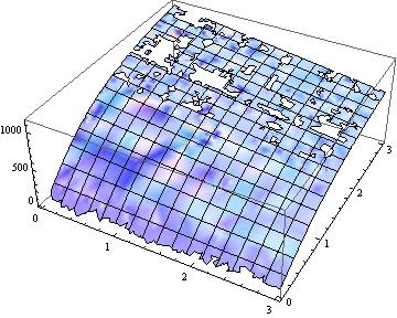
Taking into account that immaginary numbers (with tiny imaginary parts) occur,

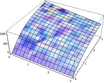
Plot3D[Re[DanLichtblau /. {a -> aa, e -> ee}], {aa, .01, 3}, {ee, .01,   3}]

is much better

Anyhow, there is a difference between the expression Dan has posted above and my result of his code: In the leading factor my sytem gets a denominator like

12 (1 + e^2)^(7/2)

Note the exponent 7 / 2 compared to 3 / 2 in Dan's post. What is the reason?

And indeed, if you use the output given by Dan the plot (Plot3D) looks completely different.

Among this double integral, "a" and "e" are assumed to be unknown parameters. I want to calculate this integral when "a" or "e" is set as a constant. And if possible, I want to draw the 3D plot of this integral with unknown "a" and "e". Thanks very much.

I speed up computation at factor 10.

 n = 1/4;(*Decrease the value to smooth a plot,the calculation time will be longer *)
 ListPlot3D[Partition[Flatten[Table[{a, e, f[a, e]}, {a, -2.01, 2, n}, {e, -2.01, 2, n}]],
 3], ColorFunction -> "SolarColors", PlotLegends -> Automatic]

regards, Mariusz

Hi

Yours $r$ variable need a value. You forgot to add it.

NIntegrate needs to be all variable constans a numeric. I'm add Method -> "LocalAdaptive" possible Integral may be singular at some values.

r=1;(* you may change this value*)
f[a_, e_, r_] := 196 Pi a - 2 (NIntegrate[Sqrt[196 - x^2], {y, 0, r Tan[e]}, {x, y/Tan[e], r}, 
Method -> "LocalAdaptive"] - (e r^3)/3) + 2 Re[NIntegrate[Sqrt[196 - x^2], {y, 0, r Tan[e] - a}, {x, (a + y)/Tan[e], r}, 
Method -> "LocalAdaptive"] - NIntegrate[Sqrt[-x^2 - y^2 + 196], {y, 0, -a Cos[e]^2 + (Sqrt[2] Sin[e])/2 Sqrt[
392 - a^2 - (a^2) Cos[2 e]]}, {x, (a + y)/Tan[e], Sqrt[14^2 - y^2]}, Method -> "LocalAdaptive"]]

n = 1/3;(*Decrease the value to smooth a plot,the calculation timewill be longer*)
ListPlot3D[Partition[Flatten[Table[{a, e, f[a, e, r]}, {a, -2.01, 2, n}, {e, -2.01, 2, n}]], 3], ColorFunction -> "SolarColors", 
PlotLegends -> Automatic]

For more information read Documentation Center it's all there,everything you need.

Regards, Mariusz