We discuss similarity and differences between interest rates forwards and futures. Differences are explained not through products mechanics, but as expectations based on different probability measures. We show that forward rates are not risk-neutral expectations of Libor rates as their measures are not identical. Several drift correction schemes are presented to show the conditions under which both rates converge.
Introduction
Futures and forwards are one of the oldest financial instruments. They represent the family of simplest derivative products and are well-known to all members of financial community. Despite being around for a long time, the question why and how they differ is still not completely understood. We therefore look at these products again and bring theoretical reasoning into the scope to show that futures and forwards are essentially different products with their own pricing dynamics driven by different probability measures. Although forwards and futures exist in various of financial classes, we focus on interest rates where this topic is most pronounced.
Zero-coupon bond as a discount factor
Time value of money is generally associated with (i) compounding and (ii) its inverse - i.e. discounting. The latter is normally associated with a discount factor - i.e. zero-coupon bond that pays unity at maturity. This is denoted as B[t,T] where t describes initiation time and T is maturity. A standard conventions assumes t=0, which translates into current discount factor B[0,T] for T>0.
Zero-coupon bond B[t,T] is not unique measure of the time value of money. Additional measure include:
A) yield
B[t,T] = Exp[-Y[t,T] ?[t,T]]
where ?[t,T] stands for the year-fraction this is unique constant rate under continuous compounding
B) term rate
B[t,T] = 1/ (1+R[t,T] ?[t,T]}
this is unique constant rate on interval t-T with no compounding. The above term rate definition above is obtained from the floating rate note (FRN) pricing formula paying Libor index with one remaining payment:
B[t,T] (1+ R[[t,T] ?[t,T]) = 1
Forward rates
When interest rates are deterministic, it can be shown that B[0,t] B[t,T] = B[0,T]. However, if they are not, this cannot be established since B[t,T] will not be known until time t (t>0). However, B[0,T] / B[0,t] is till a useful measure as it denotes forward discount factor starting at time t with final maturity at T.
Since discount factor is function of rate process, we can define associated forward rate f0[t,T] as the rate observed today for borrowing (lending) starting on time t and maturing at time T. If the agreement to lend or borrow is done on the forward rate f0[t,T], then the contract value must have present value = 0.
Clear[B, F, f0, ?];
F[t, T] = B[0, T]/B[0, t];
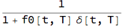
F[t, T] = 1/(1 + f0[t, T] ?[t, T])
Agreements to borrow or lend in the future (i.e. forward rate agreements) are generally done on the fixed rate K. This is essentially an agreement to exchange market term rate R[t,T] for the fixed contract rate K. This contract is priced on the assumption that the market term rate R[t,T] will be the forward rate f0[t,T]. Although R[t,T] is unknown at time 0, f0[t,T] is, so this equality allows to price the forward rate agreement at inception at time 0.
Futures
Futures contract is similar to forward, but some differences exist. It is designed to lock in a price for purchase / sell of an asset before the physical purchase / sale occurs. At the same time, future corrects certain deficiencies of the forward contract - it allows daily variation of the rate for the given delivery rate, and due to mark-to-market nature, it eliminates the counterparty exposure. Daily settlement is primary difference in these two contracts.
Future contract is associated with a future price. This is the settlement price on which contract evaluates. In the risk-neutral world governed by risk-neural probabilities, the future price is simply ? = Ern[X[T]] = Exp[r T]* P0 where P0 is the future price at time 0. When the rate is constant, the future price equals forward price.
Martingales
A process is known as martingale under the risk-neutral probabilities if it satisfies the condition: h(t) = Ern[h(T)] for t<T where Ern denotes the risk-neutral expectation. In other words, price now = Ern[price next].
This also applies to futures. Futures prices are determined by the fact the ?(t) is martingale relative to risk-neutral probabilities. In the context of risk-free world, we frequently work with money-market account which earns risk-free rate and compounds in forward time. At inception, the account is equal to A(0) = 1, and the balance at time t is A(t) = Exp[ r t] when rate stays constant. Given this, a method to determine the price of tradable asset becomes: h(t)/A(t) = Ern[h(T)/A(T)] Since zero-coupon bond is tradable security, we establish that B[t,T] / A(t) = Ern[1/A(T)]. Since A(T) = A(t)*Exp[?r(s) ds], the pricing formula for zero-coupon bond becomes B[t,T] = Ern[Exp[-?r(s) ds]].
The nature of future - forward difference
Future
Interest rate future exists in many currencies and involves 3 months contract referenced to Xibor index (eg- Libor, Euribor, Tibor etc.). At contract maturity the holder makes loan to the counterparty equal to 3-months Xibor rate. This is the term rate R[t,T] we defined in the first paragraph. The associated future price (i..e future rate) is martingale:
R0[t,T] = Ern[R[t,T]]
This means that the expected future rate is the 3-month term rate R[t,T] for the period [t,T] observed today.
Forward
We can now define the similar reasoning for the forward term rate ==> f0[t,T]. We can get its definition form the forward discount factor F[t,T]
Clear[B, f0, F]
F[t, T] = B[0, T]/B[0, t];
Solve[F[t, T] == 1/(1 + f0[t, T] \[Delta][t, T]), f0[t, T]]
soln = f0[t, T] /. %;
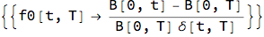
This is the forward rate obtained from the ratio of discount factors.
We split the formula above into (i) numerator and (ii) denominator and express the two zero-bonds as risk-neutral expectations of zero-rates:
num1 = Numerator[soln];
num2 = num1 /. {B[0, t] -> Exp[-Integrate[r[s], {s, 0, t}]], B[0, T] -> Exp[-Integrate[r[s], {s, 0, T}]]}
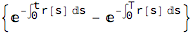
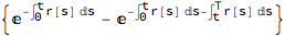
We can simplify the above using the fact that interval [0,T] can be broken into two shorter intervals [0,t] and [t,T].
num3 = num2 /. {Exp[-Integrate[r[s], {s, 0, T}]] ->
    Exp[-Integrate[r[s], {s, 0, t}]] Exp[-Integrate[r[s], {s, t, T}]]}
We rewrite the expression as follows:
num4 = Collect[num3, Exp[-Integrate[r[s], {s, 0, t}]]]
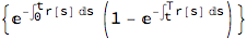
and then further simplify by bringing the year-fraction into the formula
num5 = num4 /. {Exp[-Integrate[r[s], {s, t, T}]] -> B[t, T]};
num6 = num5/?[t, T]
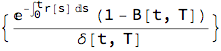
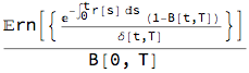
Combining all terms brings us the formula:
f0[t, T] = (1/B[0, T]) Ern[num6]
Using the definition
B[t,T] = 1/(1+R[t,T] ?[t,T])
we further state:
Clear[B, R];
B[t, T] = 1/(1 + R[t, T] ?[t, T]);
num7 = (1 - B[t, T])/?[t, T] // Simplify
which translates to
R[t,T] B[t,T]

Clear[B, R, f0];
num8 = num7 /. {R[t, T]/(1 + R[t, T] ?[t, T]) -> R[t, T]*B[t, T]} // Simplify
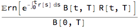
We can now express the expectation of the forward rate as:
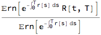
f0[t, T] = (1/B[0, T]) Ern[
   Exp[-Integrate[r[s], {s, 0, t}]] num8]
further rewrite the discount factor formula as rate process
f0[t, T] = f0[t, T] /. {B[t, T] -> Exp[-Integrate[r[s], {s, t, T}]]}
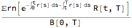
Noting that two periods combine into one [0,t] [t,T] -> [0,T]
f0[t, T] /. {Exp[-Integrate[r[s], {s, 0, t}]] Exp[-Integrate[
       r[s], {s, t, T}]] -> Exp[-Integrate[r[s], {s, 0, T}]]}
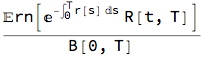
which further simplifies to:
% /. {B[0, T] -> Ern[Exp[-Integrate[r[s], {s, 0, T}]]]}
The above formula shows that the forward rate f0[t,T] is NOT the risk-neutral expectation of the Xibor term rate R[t,T]. The formula above shows that the forward rate is the expectation taken under different probability measure where the Xibor rate is weighted by Exp[-?r(s) ds].
Defining both rates in simplified notation with [DoubleStruckCapitalE] representing the risk-neutral expectation, we can now quantify the difference between the two rates:
Clear[R, f0, B];
R[t, T] = \[DoubleStruckCapitalE][R];
f0[t, T] = \[DoubleStruckCapitalE][R B]/\[DoubleStruckCapitalE][B];
f0[t, T] - R[t, T] // Together
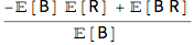
If R and B were independent, the nominator would vanish leading to the fact that forward rate = futures rate. However, independence cannot be justified since R is a rate and B is a discount factor that implies negative correlation between the two.
This will make the nominator negative, leading to a conclusion that forward rate < future term rate. This is not surprising. Since futures offer certain advantages over forwards - namely in daily settlement - their higher price relative to forwards is logical.
The adjustment of future rate to the forward rate is known as drift correction. Practitioners refer to it as 'convexity adjustment'. As the formula above shows, different dynamics for interest rates will lead to different drift correction formula.
Various drift correction approaches
We look at several examples of drift correction formulas where we assume certain distributions for the term rate R[t,T] and the discount factor B[t,T]. We set the Xibor distribution to Normal (explicitly allowing for negative rates), whereas we choose different processes for discount factor. The joint expectation is computed via Copula distributions (Binormal and Farlie-Gumbel-Morgenstern). We output (i) the joint copula expectation of rate and discount factor E[R B] and the final drift correction formula. As shown below, different combination of rate and DF processes lead to a different drift correction formulas.
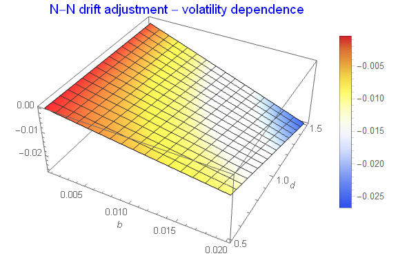
Normal- Normal process
rDist = NormalDistribution[a, b];
bDist = NormalDistribution[c, d];
bc1 = CopulaDistribution[{"Binormal", ?}, {rDist, bDist}];
jd1 = Expectation[x y, {x, y} \[Distributed] bc1,
Assumptions -> b > 0 && d > 0] // Simplify
eR = Expectation[x, x \[Distributed] rDist, Assumptions -> b > 0];
eD = Expectation[y, y \[Distributed] bDist, Assumptions -> d > 0];
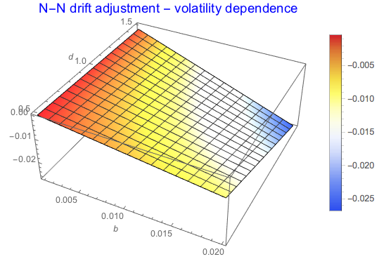
dc1 = (jd1 - eR eD)/eD // Simplify


Drift adjustment formula depends on the covariance product and DF drift. This is similar to 'quanto' adjustment in equity options.
Plot3D[dc1 /. {c -> 0.95, ? -> -0.85}, {b, 0.001, 0.02}, {d, 0.5, 1.5},
 ColorFunction -> "TemperatureMap", PlotLegends -> Automatic,
 AxesLabel -> Automatic,
 PlotLabel -> Style["N-N drift adjustment - volatility dependence", 15, Blue]]
Normal - Log Normal process
bDist = LogNormalDistribution[c, d];
bc1 = CopulaDistribution[{"Binormal", ?}, {rDist, bDist}];
jd1 = Expectation[x y, {x, y} \[Distributed] bc1,
   Assumptions -> b > 0 && d > 0] // Simplify
eR = Expectation[x, x \[Distributed] rDist, Assumptions -> b > 0];
eD = Expectation[y, y \[Distributed] bDist, Assumptions -> d > 0];
dc1 = (jd1 - eR eD)/eD // Simplify
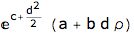

Normal - LogNormal process generates similar drift adjustment routine to the double-normal process.
Normal - Laplace process
bDist = LaplaceDistribution[c, d];
bc1 = CopulaDistribution[{"FGM", ?}, {rDist, bDist}];
jd1 = Expectation[x y, {x, y} \[Distributed] bc1,
   Assumptions -> b > 0 && d > 0] // Simplify
eR = Expectation[x, x \[Distributed] rDist, Assumptions -> b > 0];
eD = Expectation[y, y \[Distributed] bDist, Assumptions -> d > 0];
dc1 = (jd1 - eR eD)/eD // Simplify
Normal -Laplace process (as a special case of Variance-Gamma process) generates more complex adjustment rule with deeper dependence on each process.
Normal - Gamma process
bDist = GammaDistribution[c, d];
bc1 = CopulaDistribution[{"FGM", ?}, {rDist, bDist}];
jd1 = Expectation[x y, {x, y} \[Distributed] bc1,
   Assumptions -> b > 0 && d > 0 && c > 0] // Simplify
eR = Expectation[x, x \[Distributed] rDist, Assumptions -> b > 0];
eD = Expectation[y, y \[Distributed] bDist, Assumptions -> d > 0 && c > 0];
dc1 = (jd1 - eR eD)/eD // Simplify
Normal-Gamma process is well defined and relatively simple.
Normal - Logistic process
bDist = LogisticDistribution[c, d];
bc1 = CopulaDistribution[{"FGM", ?}, {rDist, bDist}];
jd1 = Expectation[x y, {x, y} \[Distributed] bc1,
   Assumptions -> b > 0 && d > 0 && -1 <= ? <= 1] // Simplify
eR = Expectation[x, x \[Distributed] rDist, Assumptions -> b > 0];
eD = Expectation[y, y \[Distributed] bDist, Assumptions -> d > 0];
dc1 = (jd1 - eR eD)/eD // Simplify


Simplicity is also a feature of Normal-Logistic process where the adjustment formula is a product of covariances
Normal - K process
bDist = KDistribution[c, d];
bc1 = CopulaDistribution[{"FGM", ?}, {rDist, bDist}];
jd1 = Expectation[x y, {x, y} \[Distributed] bc1,
   Assumptions -> b > 0 && d > 0 && -1 <= ? <= 1] // Simplify
eR = Expectation[x, x \[Distributed] rDist, Assumptions -> b > 0];
eD = Expectation[y, y \[Distributed] bDist, Assumptions -> d > 0];
dc1 = (jd1 - eR eD)/eD // Simplify

On the other hand, selection of Normal - K process (as representation of Exponential / Gamma mixture) for DF calibration leads to a complex adjustment rule
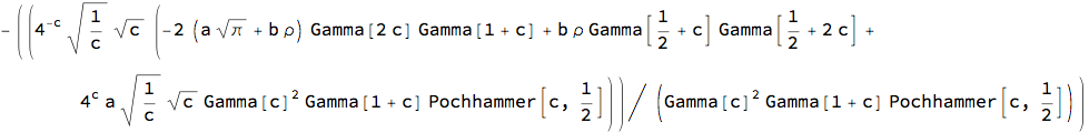
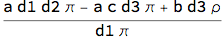
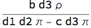
Normal - Johnson SN process
bDist = JohnsonDistribution["SN", c, d1, d2, d3];
bc1 = CopulaDistribution[{"FGM", ?}, {rDist, bDist}];
jd1 = Expectation[x y, {x, y} \[Distributed] bc1,
   Assumptions -> b > 0 && d3 > 0 && -1 <= ? <= 1] // Simplify
eR = Expectation[x, x \[Distributed] rDist, Assumptions -> b > 0];
eD = Expectation[y, y \[Distributed] bDist, Assumptions -> d3 > 0];
dc1 = (jd1 - eR eD)/eD // Simplify
Conclusion
We have taken more rigorous approach to show why futures and forwards differ when the rates are stochastic. We have demonstrated that the nature of deviation lies in probability measure - due to the fact that futures and forwards are essentially subject to different expectations. This leads to a conclusion that forward rates cannot be unbiased estimates on future Xibor rates since forward process is principally different.
We have also demonstrated that drift adjustment formula to equate futures and forward is probability-dependent, and selection of different rate (discount factor) processes leads to different results. The rule complexity depends on (i) joint expectation and (ii) distributional assumptions about each component.
We conclude the exposition to model selection with the higher-order Normal-Johnson process of 'SN' type where more process parameters provide better control for DF process.
 Attachments:


