In the interval
$0<x2<1$, the code that I mentioned above works well, here I will repeat this code for
$qmax=1$
qmax = 1; h = .05; d = 1; lam = d; a = 25*d; k = (2*Pi/d);
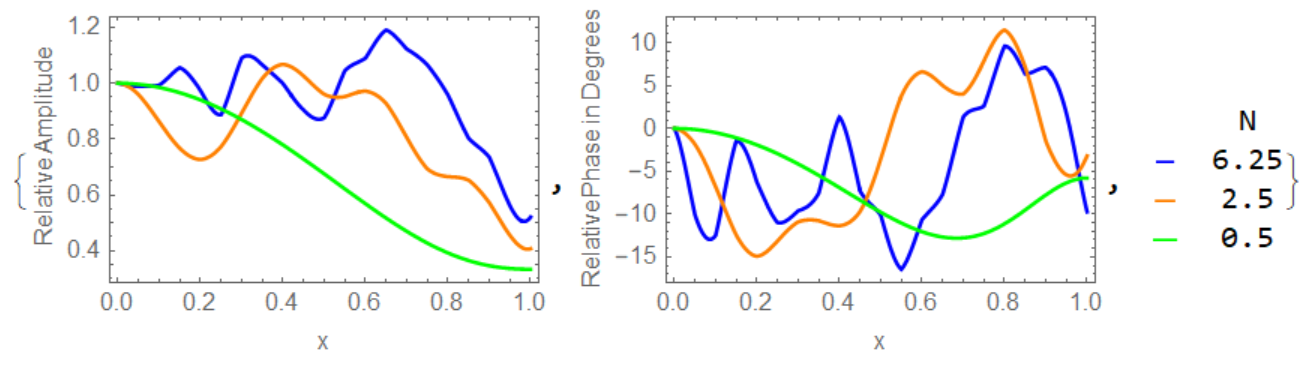
(*Fresnel number N=6.25*)
k1 = 19.635; b = (k*a^2)/(2*k1); c = a*Exp[I*(Pi/4 - k*b)]/Sqrt[lam*b];
u[0][x_] := 1; v[0][x_] := 0;
Do[{u[q] =
Interpolation[
Table[{x2,
Re[c*NIntegrate[(u[q - 1][x1] + I*v[q - 1][x1])*
Exp[-I*k1*(x1 - x2)^2], {x1, -1, 1}]]}, {x2, -1, 1, h}]],
v[q] = Interpolation[
Table[{x2,
Im[c*NIntegrate[(u[q - 1][x1] + I*v[q - 1][x1])*
Exp[-I*k1*(x1 - x2)^2], {x1, -1, 1}]]}, {x2, -1, 1,
h}]]}, {q, 1, qmax}]
p1 = Plot[
Abs[u[qmax][x] + I*v[qmax][x]]/Abs[u[qmax][0] + I*v[qmax][0]], {x,
0, 1}, Frame -> True, FrameLabel -> {"x", "Relative Amplitude"},
PlotRange -> All, PlotStyle -> Blue];
f1 = Plot[
180*(Arg[u[qmax][x] + I*v[qmax][x]] -
Arg[u[qmax][0] + I*v[qmax][0]])/Pi, {x, 0, 1}, Frame -> True,
FrameLabel -> {"x", "Relative Phase in Degrees"} ,
PlotRange -> All, PlotStyle -> Blue];
(**Fresnel number N=2.5**)
k1 = 7.85398; b = (k*a^2)/(2*k1); c =
a*Exp[I*(Pi/4 - k*b)]/Sqrt[lam*b];
u[0][x_] := 1; v[0][x_] := 0;
Do[{u[q] =
Interpolation[
Table[{x2,
Re[c*NIntegrate[(u[q - 1][x1] + I*v[q - 1][x1])*
Exp[-I*k1*(x1 - x2)^2], {x1, -1, 1}]]}, {x2, -1, 1, h}]],
v[q] = Interpolation[
Table[{x2,
Im[c*NIntegrate[(u[q - 1][x1] + I*v[q - 1][x1])*
Exp[-I*k1*(x1 - x2)^2], {x1, -1, 1}]]}, {x2, -1, 1,
h}]]}, {q, 1, qmax}]
p2 = Plot[
Abs[u[qmax][x] + I*v[qmax][x]]/Abs[u[qmax][0] + I*v[qmax][0]], {x,
0, 1}, Frame -> True, FrameLabel -> {"x", "Relative Amplitude"} ,
PlotRange -> All, PlotStyle -> Orange];
f2 = Plot[
180*(Arg[u[qmax][x] + I*v[qmax][x]] -
Arg[u[qmax][0] + I*v[qmax][0]])/Pi, {x, 0, 1}, Frame -> True,
FrameLabel -> {"x", "Relative Phase"} , PlotRange -> All,
PlotStyle -> Orange];
(***Fresnel number N=0.5***)
k1 = 1.5708; b = (k*a^2)/(2*k1); c = a*Exp[I*(Pi/4 - k*b)]/Sqrt[lam*b];
u[0][x_] := 1; v[0][x_] := 0;
Do[{u[q] =
Interpolation[
Table[{x2,
Re[c*NIntegrate[(u[q - 1][x1] + I*v[q - 1][x1])*
Exp[-I*k1*(x1 - x2)^2], {x1, -1, 1}]]}, {x2, -1, 1, h}]],
v[q] = Interpolation[
Table[{x2,
Im[c*NIntegrate[(u[q - 1][x1] + I*v[q - 1][x1])*
Exp[-I*k1*(x1 - x2)^2], {x1, -1, 1}]]}, {x2, -1, 1,
h}]]}, {q, 1, qmax}]
p3 = Plot[
Abs[u[qmax][x] + I*v[qmax][x]]/Abs[u[qmax][0] + I*v[qmax][0]], {x,
0, 1}, Frame -> True, FrameLabel -> {"x", "Relative Amplitude"} ,
PlotRange -> All, PlotStyle -> Green];
f3 = Plot[
180*(Arg[u[qmax][x] + I*v[qmax][x]] -
Arg[u[qmax][0] + I*v[qmax][0]])/Pi, {x, 0, 1}, Frame -> True,
FrameLabel -> {"x", "Relative Phase"} , PlotRange -> All,
PlotStyle -> Green];
{Show[{p1, p2, p3}], Show[{f1, f2, f3}],
Grid[{{"",
"N"}, {Graphics[{Blue, Line[{{0, 7}, {10, 7}}]},
ImageSize -> {20, 10}],
6.25}, {Graphics[{Orange, Line[{{0, 6}, {10, 6}}]},
ImageSize -> {20, 10}],
2.5}, {Graphics[{Green, Line[{{0, 5}, {10, 5}}]},
ImageSize -> {20, 10}], 0.5}}]}