Message Boards Message Boards

UNET image segmentation in stem cells research

For my research project I had to encounter a thorny problem. But before I tell about the problem I would like to briefly mention something about my research project. Basically I am using embryonic stem cells that self-organize to form spheroids (balls of cells) to study gastrulation events. In order to not bog down the readers with technical jargon, “gastrulation” is a process where the stem cells start to form the different layers; each layer then goes onto form the various tissues/organs, in the process unraveling the developmental plan of the entire organism. I am using experimental techniques and quantitative principles from biophysics and engineering to understand some aspects of this crucial process

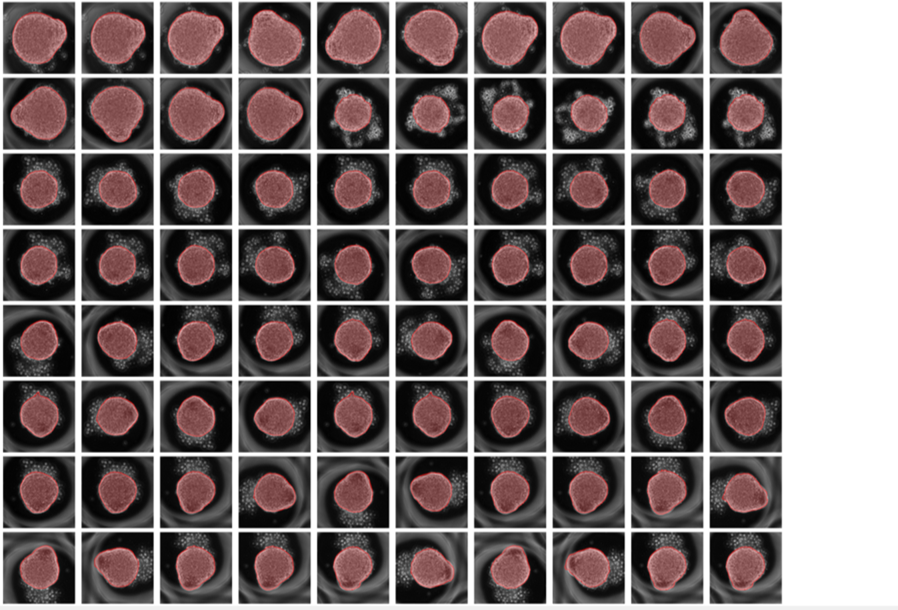
Now coming back to the problem at hand, the gastruloids (image below) are quite rough in their appearance and not as beautiful as one would like them to be (only a mother can love such an image). Any means of quantifying these gastruloids requires me to initially segment them. When you see a time-lapse images of gastruloids it becomes apparent that they shed a lot of cells (for reasons I do not know yet). This adds considerable noise to the system; oftentimes to the point that – as a human – my eyes are fooled and run into the difficulty of finding the right contours for the spheroids. Here comes the disclosure: classical means/operations in image-processing (gradients and edge detection, filtering, morphological operations etc.. ) prove utterly futile for image segmentation in my case.
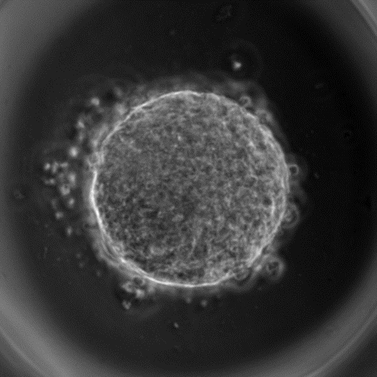
enter image description here

(A gastruloid – virtually a ball of cells with many shed around the periphery)

So what can you do to address the problem where even the best image processing tool in existence – the human eyes – fails. This is precisely where you take help of neural networks. Neural networks are selling like hotcakes during the recent years and added life and hope to the once dead area of artificial intelligence. Again to avoid underlying technical details, neural networks is a paradigm utilized by the computer to mimic the working of a human brain by taking into account the complex interactions between the cells – but only digitally. There are many flavours of neural networks out there, each one geared towards performing a specific task. With advancements made in the area of deep learning/artificial intelligence, the neural nets have started to surpass humans in tasks that humans have been known to be best for i.e. classification tasks. A few recent examples that come to mind include Google’s AlphaGo beating the former World Go champion and an AI diagnosing skin cancer with an unprecedented accuracy.

I utilized one such flavour of neural networks (a deep convolutional network – termed as UNET) to solve my longstanding problem. I constructed the network in Wolfram-Language with external help from Alexey Golyshev. UNET is a deep convolutional network that has a series of convolutional and pooling operations in the contraction phase of the net (wherein the features are extracted) and a sequence of deconvolution & convolution operations in the expansion phase which then yields an output from the network. This output can be subjected to a threshold to ultimately generate a binarized mask (the image segmentation).

enter image description here

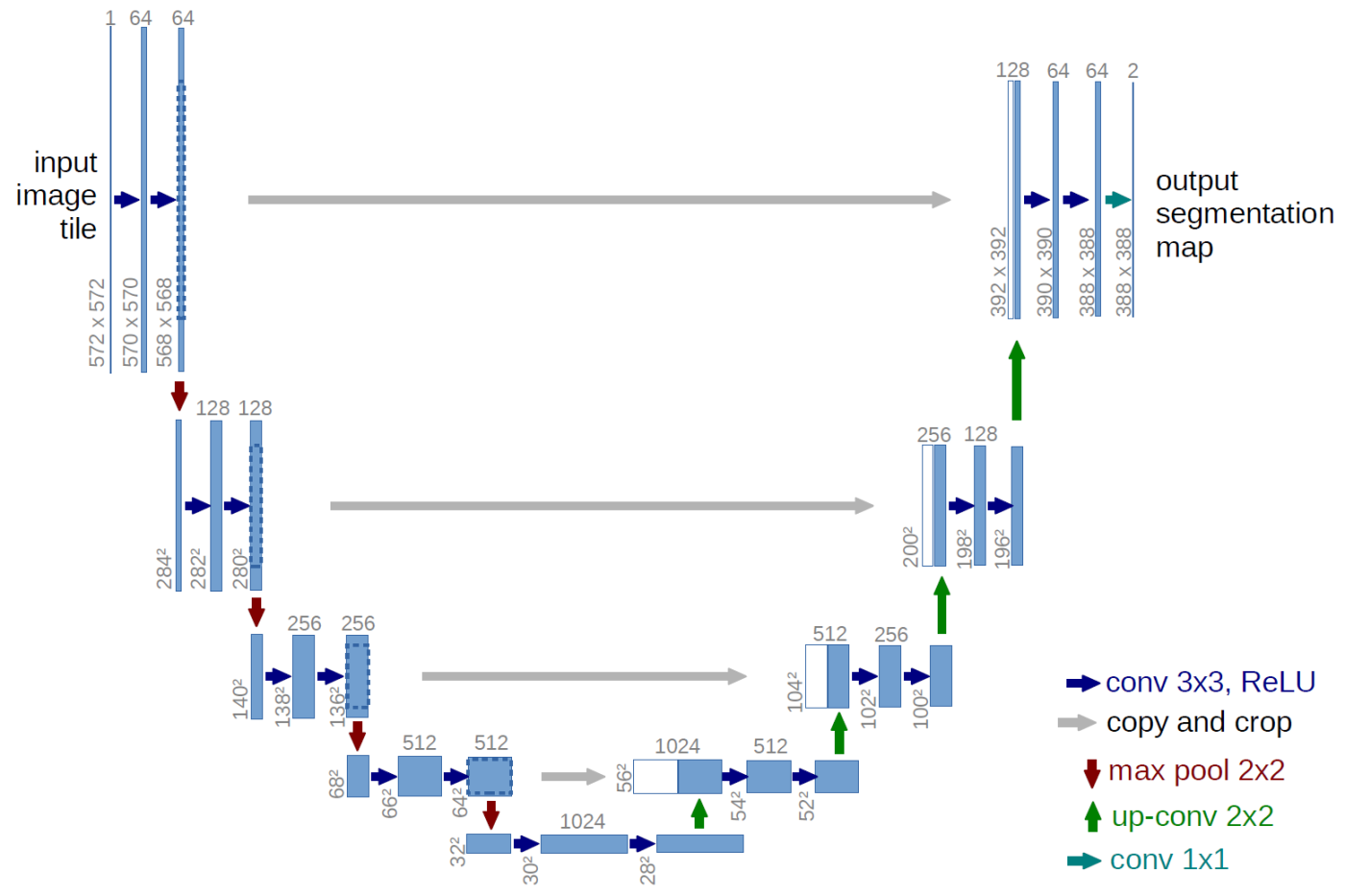
The architecture of UNET as provided by the author: https://lmb.informatik.uni-freiburg.de/people/ronneber/u-net/

(* ::Package:: *)
BeginPackage["UNETSegmentation`"]

(* ::Section:: *)
(*Creating  UNet*)

conv[n_]:=NetChain[
{
 ConvolutionLayer[n,3,"PaddingSize"->{1,1}],
 Ramp,
 BatchNormalizationLayer[],
 ConvolutionLayer[n,3,"PaddingSize"->{1,1}],
 Ramp,
 BatchNormalizationLayer[]
}
];

pool := PoolingLayer[{2,2},2];

dec[n_]:=NetGraph[
{
 "deconv" -> DeconvolutionLayer[n,{2,2},"Stride"->{2,2}],
 "cat" -> CatenateLayer[],
 "conv" -> conv[n]
},
{
 NetPort["Input1"]->"cat",
 NetPort["Input2"]->"deconv"->"cat"->"conv"
}
];

nodeGraphMXNET[net_,opt: ("MXNetNodeGraph"|"MXNetNodeGraphPlot")]:= net~NetInformation~opt;

UNET := NetGraph[
<|
"enc_1"-> conv[64],
"enc_2"-> {pool,conv[128]},
"enc_3"-> {pool,conv[256]},
"enc_4"-> {pool,conv[512]},
"enc_5"-> {pool,conv[1024]},
"dec_1"-> dec[512],
"dec_2"-> dec[256],
"dec_3"-> dec[128],
"dec_4"-> dec[64],
"map"->{ConvolutionLayer[1,{1,1}],LogisticSigmoid}
|>,
{
NetPort["Input"]->"enc_1"->"enc_2"->"enc_3"->"enc_4"->"enc_5",
{"enc_4","enc_5"}->"dec_1",
{"enc_3","dec_1"}->"dec_2",
{"enc_2","dec_2"}->"dec_3",
{"enc_1","dec_3"}->"dec_4",
"dec_4"->"map"},
"Input"->NetEncoder[{"Image",{160,160},ColorSpace->"Grayscale"}]
]

(* ::Section:: *)
(*DataPrep*)

dataPrep[dirImage_,dirMask_]:=Module[{X, masks,imgfilenames, maskfilenames,ordering, fNames,func},

func[dir_] := (SetDirectory[dir];
fNames = FileNames[];
ordering = Flatten@StringCases[fNames,x_~~p:DigitCharacter.. :> ToExpression@p];
Part[fNames,Ordering@ordering]);

imgfilenames = func@dirImage;
X = ImageResize[Import[dirImage<>"\\"<>#],{160,160}]&/@imgfilenames;
maskfilenames = func@dirMask;
masks = Import[dirMask<>"\\"<>#]&/@maskfilenames;
{X, NetEncoder[{"Image",{160,160},ColorSpace->"Grayscale"}]/@masks}
]


(* ::Section:: *)
(*Training UNet*)

trainNetwithValidation[net_,dataset_,labeldataset_,validationset_,labelvalidationset_, batchsize_: 8, maxtrainRounds_: 100]:=Module[{},
 SetDirectory[NotebookDirectory[]];
 NetTrain[net, dataset->labeldataset,All, ValidationSet -> Thread[validationset-> labelvalidationset],
 BatchSize->batchsize,MaxTrainingRounds->maxtrainRounds, TargetDevice->"GPU",
 TrainingProgressCheckpointing->{"Directory","results","Interval"->Quantity[5,"Rounds"]}]
];

trainNet[net_,dataset_,labeldataset_, batchsize_:8, maxtrainRounds_: 10]:=Module[{},
 SetDirectory[NotebookDirectory[]];
 NetTrain[net, dataset->labeldataset,All,BatchSize->batchsize,MaxTrainingRounds->maxtrainRounds, TargetDevice->"GPU",
 TrainingProgressCheckpointing->{"Directory","results","Interval"-> Quantity[5,"Rounds"]}]
];

(* ::Section:: *)
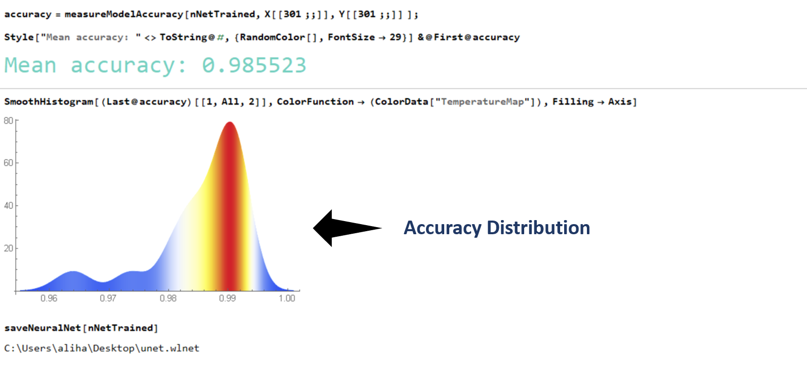
(*Measure Accuracy*)

measureModelAccuracy[net_,data_,groundTruth_]:= Module[{acc},
acc =Table[{i, 1.0 - HammingDistance[N@Round@Flatten@net[data[[i]],TargetDevice->"GPU"],
 Flatten@groundTruth[[i]]]/(160*160)},{i,Length@data}
];
{Mean@Part[acc,All,2],TableForm@acc}
];

(* ::Section:: *)
(*Miscellaneous*)

saveNeuralNet[net_]:= Module[{dir = NotebookDirectory[]},
 Export[dir<>"unet.wlnet",net]]/; Head[net]=== NetGraph;


saveInputs[data_,labels_,opt:("data"|"validation")]:=Module[{},
 SetDirectory[NotebookDirectory[]];
 Switch[opt,"data",
  Export["X.mx",data];Export["Y.mx",labels],
  "validation",
  Export["Xval.mx",data];Export["Yval.mx",labels]
 ]
]

EndPackage[];

The above code can also be found in the repository @ Wolfram-MXNET GITHUB

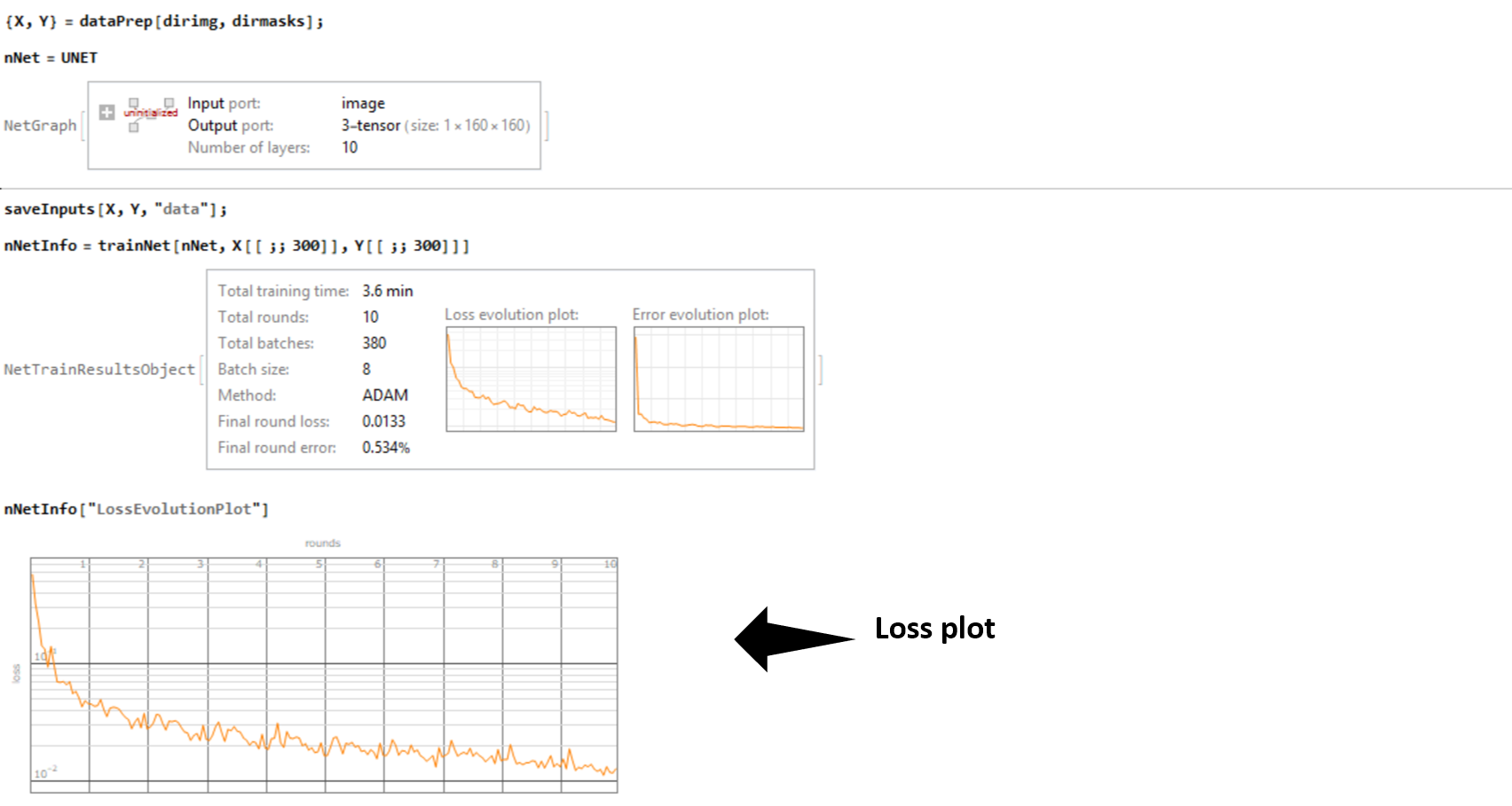
I trained my network over my laptop GPU (Nvidia GTX 1050) by feeding an augmented data (a set of 300 images constructed from a small dataset) . The training was done in under 3 minutes !. The accuracy (computed as the Hamming Distance between two vectors) of the generated binary masks with respect to the ground truth (unseen data) for a set of 90 images was 98.55 %. And with this a task that previously required me to painstakingly trace the contour of the gastruloids manually can now be performed in a matter of milliseconds. All the saved time and perspiration to be utilized somewhere else?

enter image description here

Below is the results obtained by applying our trained net on one input:

enter image description here

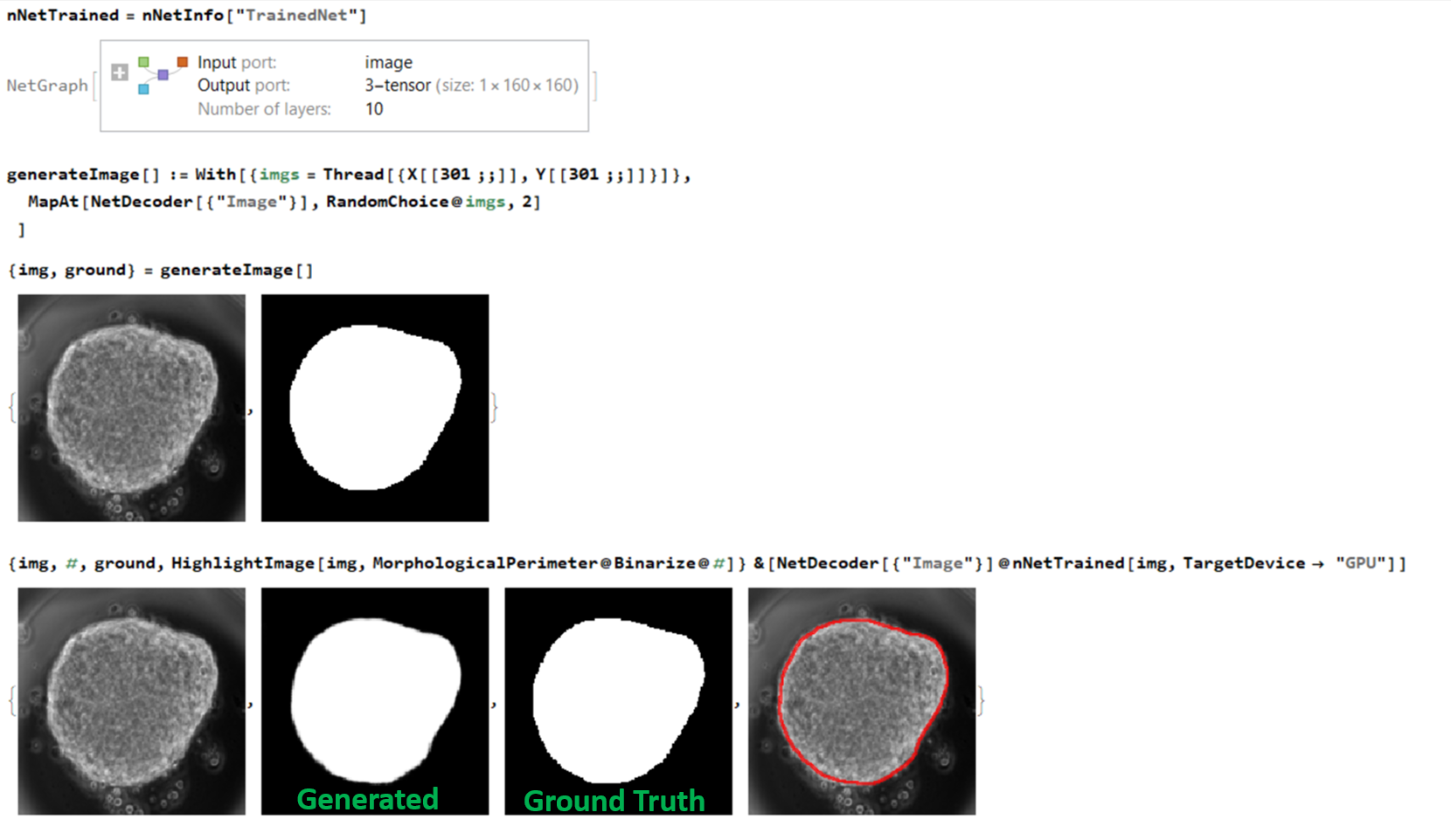
The interesting aspect for me regarding the network was that despite my gastruloids being highly dynamic (changing shape over time) I never had to explicity state it to the network. All the necessary features were learned from the limited number of images that I trained my network with. This is the beauty of the neural network.

enter image description here

Finally the output of the net as applied on a number of unseen images:

enter image description here

Note: I have a python MXNET version of UNET @ python mxnet GITHUB

The wolfram version of UNET however seems to outperform the python version even though it also utilizes MXNET at the back-end for implementing neural networks. It should not come as a surprise because my guess is that the people at Wolfram Research may have done internal optimizations on top of the library

POSTED BY: Ali Hashmi
11 Replies

Hi Ali, Martijn and Matteo

Thanks for your very valuable ideas and suggestions!

I have applied your ideas to segment human blast data and found it works excellently. Data can be found [here]. Images can easily be resized such that training works fine.

On the left side we see Human blast cells, in the middle we see the trained masks and on the right side the ground truth.

Segmentation of Images in Transmission Electron Microscopic Cell Recordings

If we want to train large data sets, I found out-of-core training by using a generating function very useful as it is described in the Wolfram Language & System Documentation Center

Many thanks!

POSTED BY: Wolfgang Hitzl

Hi Wolfgang,

I am glad it worked for you. It is very nice dataset btw. Cheers to you

POSTED BY: Ali Hashmi

Hi Wolfgang,

Looks great!!

It might be of interest to the community, i have transformed the notebook into proper paclet. With some demos and documentation. I have extended the networks with some other CONV blocks based on ResNet and others. All methods are fully generalized for 2D and 3D.

UNET

Enjoy!

POSTED BY: Martijn Froeling

Great work and very usefull!

I have generalized your network such that it can take any number of channels and classes. Your case handles one channel and one class. However i did not manage to make the single class output a binary image since the SoftmaxLayer and NetDecoder do not allow to classify one class and i did not find a suitable solution. The SoftmaxLayer with class labeling allows to give error rate feedback during the training.

pool := PoolingLayer[{2, 2}, 2];
upSamp[n_] := DeconvolutionLayer[n, {2, 2}, "Stride" -> {2, 2}]

conv[n_, p_: 0] := NetChain[{If[p == 1, pool, Nothing],
ConvolutionLayer[n, 3, "PaddingSize" -> {1, 1}], 
BatchNormalizationLayer[], Ramp,
ConvolutionLayer[n, 3, "PaddingSize" -> {1, 1}], 
BatchNormalizationLayer[], Ramp
}];

dec[n_] := NetGraph[{
"deconv" -> DeconvolutionLayer[n, {2, 2}, "Stride" -> {2, 2}],
"cat" -> CatenateLayer[],
"conv" -> conv[n]},
{NetPort["Input1"] -> "cat", 
NetPort["Input2"] -> "deconv" -> "cat" -> "conv"}
];

UNET2D[NChan_: 1, Nclass_: 1] := NetGraph[<|
"enc_1" -> conv[64], "enc_2" -> conv[128, 1], 
"enc_3" -> conv[256, 1], "enc_4" -> conv[512, 1], 
"enc_5" -> conv[1024, 1],
"dec_1" -> dec[512], "dec_2" -> dec[256], "dec_3" -> dec[128], 
"dec_4" -> dec[64],
"map" -> {ConvolutionLayer[Nclass, {1, 1}], LogisticSigmoid, 
If[Nclass > 1, TransposeLayer[{1 <-> 3, 1 <-> 2}], Nothing], 
If[Nclass > 1, SoftmaxLayer[], Nothing], 
If[Nclass > 1, Nothing, FlattenLayer[1]]}
|>,
{NetPort["Input"] -> 
"enc_1" -> "enc_2" -> "enc_3" -> "enc_4" -> "enc_5",
{"enc_4", "enc_5"} -> "dec_1", {"enc_3", "dec_1"} -> "dec_2",
{"enc_2", "dec_2"} -> "dec_3", {"enc_1", "dec_3"} -> "dec_4", 
"dec_4" -> "map"},
"Input" -> {NChan, 128, 128}, 
"Output" -> 
If[Nclass > 1, 
NetDecoder[{"Class", "Labels" -> Range[1, Nclass], 
"InputDepth" -> 3}], Automatic]
]

I also made the IuO function a bit faster for large data-sets and it reports the values per calss

ClassIOU[predi_, gti_, class_] := 
 Block[{posN, posP, fn, tp, fp, denom},
  (*find posisions as unitvector*)
  posN = Unitize[predi - class];
  posP = 1 - posN;

  (*get the values*)
  fn = Count[Pick[gti, posN, 1], class];
  tp = Count[Pick[gti, posP, 1], class];
  fp = Total[posP] - tp;

  (*if case does not exist in all data return 1*)
  denom = (tp + fp + fn);
  If[denom == 0, 1., N[tp/denom]]
  ]

IOU[pred_, gt_, nClasses_] := Block[{predf, gtf},
  predf = Flatten[pred];
  gtf = Flatten[gt];
  Table[ClassIOU[predf, gtf, c], {c, nClasses}]
  ]

To split the available data into training, validation and testing data I made this function.

SplitTestData[data_, label_, ratio_: {0.7, .2, .1}] := 
 Block[{allData, train, valid, test, testData, testLabel, s1, s2, s3},
  (*Randomize data*)
  allData = RandomSample[Thread[data -> label]];

  (*split data*)      
  Print["Nuber of Samples in each set: ", Round[ratio Length[allData]]];
  {s1, s2, s3} = Accumulate@Round[ratio Length[allData]];

  (*make training validation and test data*)
  train = allData[[1 ;; s1]];
  valid = allData[[s1 + 1 ;; s2]];
  test = allData[[s2 + 1 ;;]];
  testData = test[[All, 1]];
  testLabel = test[[All, 2]];

  (*define the output*)
  {train, valid, testData, testLabel}
  ]

These are some generated test dataset on which i tested the network

  • single channel - single class

1-1

  • single channel - 2 class

1-2

  • single channel - multi class

1-n

  • multi channel - multi class

n-n

These were the results

  • single channel - single class

case1

  • single channel - 2 classes {1 -> Background, 2 -> segmentation}

case2

  • single channel - multi class {1 -> Background, 2...n -> segmentation}

case3

  • multi channel - multi class {1 -> Background, 2...n -> segmentation}

case4

And finally of course my real application to segment the heart wall from multi modal MRI contrasts. However id do have to admit that my manual annotations could be a bit better such that the network can train more accurately. (Red - Manual annotation, Blue - Trained net, Green - overlap of the two)

real data

Attachments:
POSTED BY: Martijn Froeling

Hi Martijn,

Great stuff generalizing the network !! Could you kindly attach your notebook here with the sections (single class vs. multi-class) arranged separately. Many thanks !

POSTED BY: Ali Hashmi

I have attached the notebook. It also contains the code to generate the test images.

POSTED BY: Martijn Froeling

Great! As a developer in the Wolfram ML team, it's always gratifying to see people doing interesting stuff with what we provide.

There are a couple of comments i'd ike to make about this:

First, you evaluate the final performance using the pixelwise accuracy, but in semantic segmentation there is a more informative measure, namely mean intersection over union (IoU). Geometrically, that corresponds with measuring intersection / union ratio of the "blobs" corresponding to a fixed class in the prediction and ground truth masks, and then averaging those ratios for all classes. In formulas, for a given image:

$$IoU_{c} = \frac{TP_c}{TP_c + FP_c + FN_c}$$ $$IoU = Mean(IoU_c)$$

Where c is a class and TPc, FPc and FN_c are, respectively, the number of true positive, false positive and false negative predictions for class c. The true positives give you the measure of the blob intersections, while the sum gives you the union. A reasonable (but probably not the best) implementation of IoU might be:

classIOU[pred_, gt_, class_] := 
 Block[{positionP, positionN, tp, fp, fn},
  positionP = Position[pred, class];
  positionN = Delete[Range@Length[pred], positionP];
  positionP = Flatten[positionP];
  tp = Count[gt[[positionP]], class];
  fp = Length[positionP] - tp;
  fn = Count[gt[[positionN]], class];
  N[tp/(tp + fp + fn)]
  ]
IOU[pred_, gt_, nClasses_] := Mean@Table[classIOU[pred, gt, c], {c, nClasses}]

This assumes that your data is flattened and your classes are identified with integers starting from 1.

In general, IoU is preferable to pixel accuracy because it makes up for class imbalances in the masks by averaging class-wise accuracies. Suppose, in a 1-D example, that "1" is background and "2" is gastruloid, and your prediction and ground truth masks look like this:

pred = {1, 1, 1, 1, 1, 1, 1, 1, 1, 1}
groundTruth = {1, 1, 1, 1, 2, 1, 1, 1, 1, 1} 

Pixel-level accuracy would be 90% here, but IoU gives you 45% (90% for background, 0% for gastruloid classes), because you completely failed to segment the gastruloid. Then, in you particular case, looks like you have a good balancing between background and object pixels in your data, so IoU shouldn't be far from pixelwise accuracy.

The second comment is just a technical one: when evaluating the accuracy you run the trained network in a Table, i.e. on each input separately. The framework also supports batch evaluation (or listable, if you want to say it à la WL). In this case, our neural network framework will figure out a suitable parallelization strategy and the computation will be much faster than a serial one. So you could, more efficiently, pre-compute net[data] outside the table and then compare it with the ground truths.

Again, congratulations for your work, the results look very good!

Thanks Matteo for the valuable input and the encouraging remarks. I will at some point replace the Hamming Distance criterion with the one you are proposing for gauging accuracy. Regarding your second comment, I realized it a few days back but I just felt lazy to make the change :)

POSTED BY: Ali Hashmi

enter image description here - Congratulations! This post is now a Staff Pick as distinguished by a badge on your profile! Thank you, keep it coming!

POSTED BY: Moderation Team
Posted 6 years ago

Fantastic! What gave you the idea of using UNET for this? Did you try some of the networks on the neural net repository as well? I doubt you'd get meaningful increases in accuracy, I'm just curious!

POSTED BY: Carl Lange

Thanks a lot Carl. Actually I did not know if there are nets available in the repository for segmentation. The repository is very cool btw !

POSTED BY: Ali Hashmi
Reply to this discussion
Community posts can be styled and formatted using the Markdown syntax.
Reply Preview
Attachments
Remove
or Discard

Group Abstract Group Abstract