Cross-posted from Mathematica.StackExchange

Motivation

Mathematica ships a variety of linear solvers through the interface

LinearSolve[A, b, Method -> method]

the most notable for sparse matrix A being:

• "Multifrontal" - the default solver for sparse arrays; direct solver based on a spare LU-factorization performed with UMFPACK. Big advantage: LinearSolve[A] creates a LinearSolveFunction object that can be reused.

• "Cholesky" - a direct solver using the sparse Cholesky-factorization provided by TAUCS. Also produces a LinearSolveFunction but limited to positive-definite matrices.

• "Pardiso" - a parallelized direct solver from the Intel MKL; undocumented but much faster and not nearly as memory hungry as "Multifrontal". LinearSolve[A, Method -> "Pardiso"] creates a reusable LinearSolveFunction object as well. The original Intel MKL Pardiso solver can do quite a lot more! Unfortunately, many of its features such as reusing symbolic factorizations are not accessible via LinearSolve. (Or are they? That would be great to know!)

• "Krylov" with the submethods "ConjugateGradient", "GMRES", and "BiCGSTAB" - iterative solvers that require good preconditioners and good starting values. These are supposed to work quite well for transient PDEs with smoothly varying coefficients.

See this site for reference. (It is a bit outdated but I don't think that any essential changes were made in the meantime - apart from "Pardiso".).

I mostly use linear solvers to solve PDEs, mostly elliptic ones, but also parabolic ones every now and then. On the one hand, the direct solvers hit the wall when dealing with meshes with several million degrees of freedom. And in particular, if the meshes are 3-dimensional, factorization times explode due to the high fill-in. On the other hand, the iterative solvers within Mathematica -- if I am honest -- perform so poorly on elliptic problems that I used to question the mental sanity of several numericists who told me that I had to use an iterative solver for every linear system of size larger than $5 \times 5$.

Some time ago, I learned that the really big thing would be multigrid solvers. So I wonder wether one can implement such a solver in Mathematica (be it in the native language or via LibraryLink) and how it would compare to the built-in linear solvers.

Background

Details about multigrid solvers can be found in this pretty neat script by Volker John. That's basically the source from which I drew the information to implement the V-cycle solver below.

In a nutshell, a multigrid solver builds on two ingredients: A hierarchy of linear systems (with so-called prolongation operators mapping between them) and a family of smoothers.

Implementation

CG-method as smoother

I use an iterative conjugate-gradient solver as smoother. For some reason, Mathematica's conjugate-gradient solver has an exorbitantly high latency, so I use my own implementation which I wrote several years ago. It's really easy to implement; all necessary details can be found, e.g., here. Note that my implementation returns an Association that also provides some information on the solving process. (In particular for transient PDE with varying coefficients, the number of needed iterations is often a valuable information that one might want to use for determining wether the preconditioner has to be updated.)

Options[CGLinearSolve] = {
   "Tolerance" -> 10^(-8),
   "StartingVector" -> Automatic,
   MaxIterations -> 1000,
   "Preconditioner" -> Identity
   };

CGLinearSolve[A_?SquareMatrixQ, b_?MatrixQ, opts : OptionsPattern[]] :=
   CGLinearSolve[A, #, opts] & /@ Transpose[b]

CGLinearSolve[A_?SquareMatrixQ, b_?VectorQ, OptionsPattern[]] :=
  Module[{r, u, ?, ?0, p, ?, ?old, 
    z, ?, ?, x, TOL, iter, P, precdata, normb, maxiter},
   P = OptionValue["Preconditioner"];
   maxiter = OptionValue[MaxIterations];
   normb = Sqrt[b.b];
   If[Head[P] === String,
    precdata = SparseArray`SparseMatrixILU[A, "Method" -> P];
    P = x \[Function] SparseArray`SparseMatrixApplyILU[precdata, x];
    ];
   If[P === Automatic,
    precdata = SparseArray`SparseMatrixILU[A, "Method" -> "ILU0"];
    P = x \[Function] SparseArray`SparseMatrixApplyILU[precdata, x];
    ];
   TOL = normb OptionValue["Tolerance"];
   If[OptionValue["StartingVector"] === Automatic,
    x = ConstantArray[0., Dimensions[A][[2]]];
    r = b
    ,
    x = OptionValue["StartingVector"];
    r = b - A.x;
    ];
   z = P[r];
   p = z;
   ? = r.z;
   ?0 = ? = Sqrt[r.r];
   iter = 0;
   While[? > TOL && iter < maxiter,
    iter++;
    u = A.p;
    ? = ?/(p.u);
    x = x + ? p;
    ?old = ?;
    r = r - ? u;
    ? = Sqrt[r.r];
    z = P[r];
    ? = r.z;
    ? = ?/?old;
    p = z + ? p;
    ];
   Association[
    "Solution" -> x,
    "Iterations" -> iter,
    "Residual" -> ?,
    "RelativeResidual" -> Quiet[Check[?/?0, ?]],
    "NormalizedResidual" -> Quiet[Check[?/normb, ?]]
    ]
   ];

Weighted Jacobi smoother

The weighted Jacobi method is a very simply iterative solver that employs Richardson iterations with the diagonal of the matrix as preconditioner (the matrix must not have any zero elements on the diagonal!) and a bit of damping. Works in general only for diagonally dominant matrices and positive-definite matrices (if the "Weight" is chosen sufficiently small). It's not really bad but it is not excellent either. In the test problem below, it usually necessitates one more V-cycle as the CG smoother.

Options[JacobiLinearSolve] = {
   "Tolerance" -> 10^(-8),
   "StartingVector" -> Automatic,
   MaxIterations -> 1000,
   "Weight" -> 2./3.
   };

JacobiLinearSolve[A_?SquareMatrixQ, b_?MatrixQ, opts : OptionsPattern[]] := 
  JacobiLinearSolve[A, #, opts] & /@ Transpose[b]

JacobiLinearSolve[A_?SquareMatrixQ, b_?VectorQ, OptionsPattern[]] := 
  Module[{?, x, r, ?d, dd, iter, ?, ?0, normb, TOL, maxiter},
   ? = OptionValue["Weight"];
   maxiter = OptionValue[MaxIterations];
   normb = Max[Abs[b]];
   TOL = normb OptionValue["Tolerance"];
   If[OptionValue["StartingVector"] === Automatic,
    x = ConstantArray[0., Dimensions[A][[2]]];
    r = b;
    ,
    x = OptionValue["StartingVector"];
    r = b - A.x;
    ];
   ?d = ?/Normal[Diagonal[A]];
   ? = ?0 = Max[Abs[r]];
   iter = 0;
   While[? > TOL && iter < maxiter,
    iter++;
    x += ?d r;
    r = (b - A.x);
    ? = Max[Abs[r]];
    ];
   Association[
    "Solution" -> x,
    "Iterations" -> iter,
    "Residual" -> ?,
    "RelativeResidual" -> Quiet[Check[?/?0, ?]],
    "NormalizedResidual" -> Quiet[Check[?/normb, ?]]
    ]
   ];

Setting up the solver

Next is a function that takes the system matrix Matrix and a family of prologation operators Prolongations and creates a GMGLinearSolveFunction object. This object contains a linear solving method for the deepest level in the hierarchy, the prolongation operators, and - derived from Matrix and Prolongations - a linear system matrix for each level in the hierarchy.

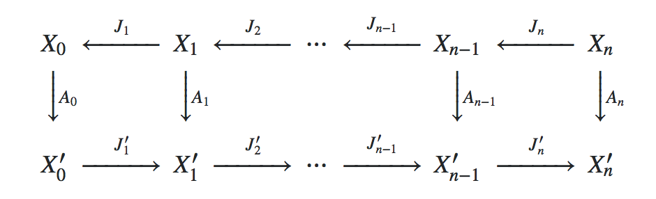
As it is the core idea of Galerkin schemes in FEM, we interpret the system matrix Matrix on the finest grid as a linear operator $A_0 \colon X_0 \to X_0'$, where $X_0$ denotes the finite element function space of continuous, piecwise-linear functions on the finest mesh and $X_0'$ denotes its dual space. Denoting the finite element function space on the $i$-th subgrid by $X_i$ and interpreting the prolongation operators in the list Prolongations as linear embeddings $J_i \colon X_{i} \hookrightarrow X_{i-1}$, we obtain the linear operators $A_i \colon X_i \to X_i'$ by Galerkin subspace projection injection, i.e. by requiring that the following diagram is commutative:

Per default, LinearSolve is used as solver for the coarsest grid, but the user may specify any other function F via the option "CoarsestGridSolver" -> F.

Some pretty-printing for the created GMGLinearSolveFunction objects is also added.

GMGLinearSolve[
   Matrix_?SquareMatrixQ,
   Prolongations_List,
   OptionsPattern[{
     "CoarsestGridSolver" -> LinearSolve
     }]
   ] := Module[{A},
   (*Galerkin subspace projections of the system matrix*)
   A = FoldList[Transpose[#2].#1.#2 &, Matrix, Prolongations];
   GMGLinearSolveFunction[
    Association[
     "MatrixHierarchy" -> A,
     "Prolongations" -> Prolongations,
     "CoarsestGridSolver" -> OptionValue["CoarsestGridSolver"][A[[-1]]],
     "CoarsestGridSolverFunction" -> OptionValue["CoarsestGridSolver"]
     ]
    ]
   ];

GMGLinearSolveFunction /: MakeBoxes[S_GMGLinearSolveFunction, StandardForm] := 
  BoxForm`ArrangeSummaryBox[GMGLinearSolveFunction, "", 
   BoxForm`GenericIcon[LinearSolveFunction],
   {
    {
     BoxForm`MakeSummaryItem[{"Specified elements: ", 
       Length[S[[1, "MatrixHierarchy", 1]]["NonzeroValues"]]}, 
      StandardForm]
     },
    {
     BoxForm`MakeSummaryItem[{"Dimensions: ", 
       Dimensions[S[[1, "MatrixHierarchy", 1]]]}, StandardForm],
     BoxForm`MakeSummaryItem[{"Depth: ", 
       Length[S[[1, "MatrixHierarchy"]]]}, StandardForm]
     }
    },
   {
    BoxForm`MakeSummaryItem[{
      Invisible["Dimensions: "],
      Column[Dimensions /@ S[[1, "MatrixHierarchy", 2 ;;]]]},
     StandardForm],
    BoxForm`MakeSummaryItem[{
      "CoarsestGridSolver: ",
      S[[1, "CoarsestGridSolverFunction"]]
      }, StandardForm]
    },
   StandardForm, "Interpretable" -> False
   ];

The solver

The following is the actual V-cycle solver. To my own surpise, the algorithm was not that hard to implement. As always, most work had to be invested into the user interface (and its still not complete as it lacks bulletproofing against 1D-10T errors).

Actually, this V-cycle solver is a purely algebraic solver (AMG); the geometry in "geometric multigrid solver" lies within the way the matrix hierarchie was constructed (namely by geometrically nested grids and Galerkin subspace methods).

Options[GMGLinearSolveFunction] = {
   "StartingVector" -> Automatic,
   "Tolerance" -> 1. 10^-8,
   "MaxIterations" -> 25,
   "StartingVectorSmoothingCounts" -> 12,
   "PreSmoothingCounts" -> 8,
   "PostSmoothingCounts" -> 8,
   "Smoother" -> Function[
     {A, b, x0, ?, p},
     (
      CGLinearSolve[A, b,
        MaxIterations -> ?,
        "StartingVector" -> x0,
        "Tolerance" -> 10^-12
        ]["Solution"]
      )
     ],
   "SmootherParameters" -> None
   };

GMGLinearSolveFunction /: GMGLinearSolveFunction[a_Association][
   Rhs_?VectorQ,
   opts0 : OptionsPattern[]
   ] := With[{
    J = a["Prolongations"],
    A = a["MatrixHierarchy"],
    Asol = a["CoarsestGridSolver"]
    },
   Module[{smoother, Rhsnorm, p, n, v, f, depth, allocationtime, startingvector, startingvectortime, solvetime, startingvectorresidual, residual, ?0, ?1, ?2, tol, maxiter, iter, opts},
    opts = Merge[{
       Options[GMGLinearSolveFunction],
       opts0
       }, Last
      ];
    n = Length /@ A;
    depth = Length[n];

    smoother = opts["Smoother"];
    p = opts["SmootherParameters"];
    If[p === None, p = ConstantArray[{}, depth];];

    (* allocate memory for computations *)

    allocationtime = AbsoluteTiming[
       v = ConstantArray[0., #] & /@ n;
       f = Join[{Rhs}, ConstantArray[0., #] & /@ Most[n]];
       ][[1]];

    (* compute starting vector *)

    startingvectortime = AbsoluteTiming[
       If[VectorQ[opts["StartingVector"]],
        v[[1]] = opts["StartingVector"];
        ,
        If[opts["StartingVector"] =!= "Null", opts["StartingVector"] == Automatic];];

       If[opts["StartingVector"] === Automatic,
        Module[{b},
          ?0 = opts["StartingVectorSmoothingCounts"];
          If[! ListQ[?0], ?0 = If[IntegerQ[?0], ConstantArray[?0, Length[n] - 1], ?0 /@ Range[depth]]];
          b = FoldList[#1.#2 &, Rhs, J];
          v[[depth]] = Asol[b[[depth]]];

          Do[v[[i]] = smoother[A[[i]], b[[i]], J[[i]].v[[i + 1]], ?0[[i]], p[[i]]], {i, depth - 1, 1, -1}];
          ];
        ,
        ?0 = None;
        ];
       ][[1]];
    startingvector = v[[1]];
    residual = startingvectorresidual = Max[Abs[Rhs - A[[1]].startingvector]];

    (* perform V-cycles until tolerance is met *)

    solvetime = AbsoluteTiming[
       ?1 = opts["PreSmoothingCounts"];
       If[! ListQ[?1], ?1 = If[IntegerQ[?1], ConstantArray[?1, Length[n] - 1], ?1 /@ Range[depth]]];
       ?2 = opts["PostSmoothingCounts"];
       If[! ListQ[?2], ?2 = If[IntegerQ[?2], ConstantArray[?2, Length[n] - 1], ?2 /@ Range[depth]]];
       Rhsnorm = Max[Abs[Rhs]];
       tol = opts["Tolerance"] Rhsnorm;
       maxiter = opts["MaxIterations"];
       iter = 0;
       While[
        residual > tol && iter < maxiter,
        iter++;
        Do[
         v[[i]] = smoother[A[[i]], f[[i]], N[Boole[i == 1]] v[[i]], ?1[[i]], p[[i]]];
         f[[i + 1]] = (f[[i]] - A[[i]].v[[i]]).J[[i]],
         {i, 1, depth - 1}];

        (* solve at deepest level with "CoarsestGridSolver" *)

         v[[depth]] = Asol[f[[depth]]];

        Do[
         v[[i]] = smoother[A[[i]], f[[i]], v[[i]] + J[[i]].v[[i + 1]], ?2[[i]], p[[i]]],
         {i, depth - 1, 1, -1}];
        residual = Max[Abs[Subtract[Rhs, A[[1]].v[[1]]]]];
        ];
       ][[1]];

    Association[
     "Solution" -> v[[1]],
     "StartingVectorResidual" -> startingvectorresidual,
     "StartingVectorNormalizedResidual" -> 
      startingvectorresidual/Rhsnorm,
     "Residual" -> residual,
     "NormalizedResidual" -> residual/Rhsnorm,
     "SuccessQ" -> residual < tol,
     "Timings" -> Dataset@Association[
        "Total" -> allocationtime + startingvectortime + solvetime,
        "Allocation" -> allocationtime,
        "StartingVector" -> startingvectortime,
        "V-Cycle" -> solvetime
        ],
     "V-CycleCount" -> iter,
     "SmootingCounts" -> Dataset@Association[
        "StartingVector" -> {?0},
        "Pre" -> {?1},
        "Post" -> {?2}
        ],
     "StartingVector" -> startingvector,
     "Smoother" -> smoother,
     "Depth" -> depth
     ]
    ]
   ];

Applications

2D Example

What we need now is a test case! Just by chance, I have recently updated my Loop subdivision routine such that it also returns the subdivision matrix if we ask kindly. We can use these subdivision matrices as prolongation operators!

So, let's start with a rather coarse mesh on the unit disk and refine it by Loop subdivision (you will need the code for LoopSubdivide if you want to try this):

R = DiscretizeRegion[Disk[], MaxCellMeasure -> 0.001];
depth = 5;
{R, J} = {Last[#1], Reverse[Rest[#2]]} & @@ 
   Transpose@NestList[LoopSubdivide, {R, {{0}}}, depth - 1];

Let's solve the following elliptic problem with Neumann boundary conditions on the disk $\varOmega$:

$$\begin{array}{rcll} (\varepsilon - \Delta) \, u &= &f, & \text{in $\varOmega\setminus \partial \varOmega$,}\\ \nu \,u&= &0, & \text{on $\partial \varOmega$.} \end{array}$$

We can use Mathematica's FEM capacities to assemble the system matrix and the right hand side for us:

f = X \[Function] 16. Sinc[4. Pi Sqrt[Abs[Dot[X + 0.5, X + 0.5]]]] - 16. Sinc[4. Pi Sqrt[Abs[Dot[X - 0.5, X - 0.5]]]] + N[Sign[X[[2]]]] + N[Sign[X[[1]]]];
fvec = Map[f, MeshCoordinates[R]];

Needs["NDSolve`FEM`"]
Rdiscr = ToElementMesh[
   R,
   "MeshOrder" -> 1,
   "NodeReordering" -> False,
   MeshQualityGoal -> 0
   ];
vd = NDSolve`VariableData[{"DependentVariables", "Space"} -> {{u}, {x, y}}];
sd = NDSolve`SolutionData[{"Space"} -> {Rdiscr}];
cdata = InitializePDECoefficients[vd, sd,
   "DiffusionCoefficients" -> {{-IdentityMatrix[2]}}, 
   "MassCoefficients" -> {{1}}, "LoadCoefficients" -> {{f[{x, y}]}}];
bcdata = InitializeBoundaryConditions[vd  sd, {DirichletCondition[u[x, y] == 0., True]}];
mdata = InitializePDEMethodData[vd, sd];
dpde = DiscretizePDE[cdata, mdata, sd];

{b, L, damping, M} = dpde["All"];
b = Flatten[Normal[b]];
A = L + 0.0001 M;

Now we create a GMGLinearSolveFunction object and solve the equation:

S = GMGLinearSolve[A, J]; // AbsoluteTiming // First
xGMG = S[b,
      "Tolerance" -> 1. 10^-8,
      "StartingVectorSmoothingCounts" -> 12,
      "PreSmoothingCounts" -> 8,
      "PostSmoothingCounts" -> 8
      ]["Solution"]; // AbsoluteTiming // First

0.835408

1.04969

Timings

Here are the timings for some other solvers:

xKrylov = LinearSolve[A, b, Method -> {
       "Krylov",
       "Method" -> "ConjugateGradient",
       "Preconditioner" -> "ILU0"
       }]; // AbsoluteTiming // First
xTAUCS = LinearSolve[A, b, "Method" -> "Cholesky"]; // AbsoluteTiming // First
xUMFPACK = LinearSolve[A, b]; // AbsoluteTiming // First
xPardiso = LinearSolve[A, b, "Method" -> "Pardiso"]; // AbsoluteTiming // First

67.948

6.89134

6.0961

2.30715

Three things to observe here:

1. Mathematica's "ConjugateGradient" is the absolute looser here. (But don't ask me for "GMRES" or "BiCGSTAB"; I was not in the mood of waiting for them.)

2. "Cholesky" cannot convert its limitation to positive-definite matrices into any advantage. That's also why I never it.

3. GMGLinearSolve is actually a bit faster than "Pardiso".

Errors

Here are the errors; I use the UMFPACK 's solution as "ground truth" (it doesn't matter, though).

Max[Abs[xUMFPACK - xGMG]]
Max[Abs[xUMFPACK - xTAUCS]]
Max[Abs[xUMFPACK - xPardiso]]
Max[Abs[xUMFPACK - xKrylov]]

3.90012*10^-10

1.14953*10^-9

2.45955*10^-10

6.27234*10^-10

They all have comparable accuracy. So, this simple multigrid solver, implemented within a long afternoon, seems to be at least on par with Pardiso. Not bad, is it?

Multiple solves are still faster with direct solvers on 2D grids

Once the factorizations of the direct solvers are computed and stored in LinearSolveFunction objects, the actual solves (triangle forward and backward substitutions) are much faster. Note that this is not necessarily the usage spectrum of iterative methods. Anyways, here are some timings:

solUMFPACK = Quiet[LinearSolve[A]]; // AbsoluteTiming // First
xUMFPACK = solUMFPACK[b]; // AbsoluteTiming // First
solTAUCS = LinearSolve[A, "Method" -> "Cholesky"]; // AbsoluteTiming // First
xTAUCS = solTAUCS[b]; // AbsoluteTiming // First
solPardiso = LinearSolve[A, "Method" -> "Pardiso"]; // AbsoluteTiming // First
xPardiso = solPardiso[b]; // AbsoluteTiming // First

6.07364

0.142823

7.28346

0.183195

2.13817

0.236214

Note that I used Quiet for UMFPACK because it complains about a bad condition number of the system and the error handling would add about 20(!) seconds to the timings. There is however no problem with the numerical errors:

Max[Abs[xGMG - xUMFPACK]]
Max[Abs[xGMG - xTAUCS]]
Max[Abs[xGMG - xPardiso]]

3.90012*10^-10

7.59533*10^-10

1.44077*10^-10

3D Example

The problem with direct solvers is that starting in 3 dimensions, their performance for dealing with matrices stemming from PDEs drops rapidly. This is why I wanted to show at least one 3-dimensional example. As there is no immediate analogon for Loop subdivision of tetrahedral meshes, I use hexahedral meshes instead.

Preparation

Here are some helper functions for generating the grid hierachy and the prolongation mappings. Prolongation is performed by hex-wise trilinear interpolation. This fits well since we are going to use first-order meshes.

Needs["NDSolve`FEM`"]
cubemesh[n_] := Module[{R},
  R = ArrayMesh[ConstantArray[1, ConstantArray[n, 3]], DataRange -> ConstantArray[{0, 1}, 3]];
  ToElementMesh[
   "Coordinates" -> MeshCoordinates[R],
   "MeshElements" -> {HexahedronElement[ MeshCells[R, 3, "Multicells" -> True][[1, 1]]]},
   "MeshOrder" -> 1, "NodeReordering" -> False, MeshQualityGoal -> 0
   ]
  ]

getEdges = Compile[{{i, _Integer}, {idx, _Integer, 1}},
   Table[{i, Compile`GetElement[idx, j]}, {j, 1, Length[idx]}],
   CompilationTarget -> "C",
   RuntimeAttributes -> {Listable},
   Parallelization -> True,
   RuntimeOptions -> "Speed"
   ];

getProlongationOperator[Rfine_ElementMesh, Rcoarse_ElementMesh, h_] :=
   Module[{pfine, pcoarse},
   pfine = Rfine["Coordinates"];
   pcoarse = Rcoarse["Coordinates"];
   #/Total[#, {2}] &@SparseArray[
     Join @@ getEdges[
        Range[Length[pfine]],
        Nearest[pcoarse -> Automatic, pfine, {?, h 1.1}, 
         DistanceFunction -> ChessboardDistance]
        ] -> 1.,
     {Length[pfine], Length[pcoarse]}, 0.
     ]
   ];

This creates the actual grid hierarchy and the prolongation mappings.

dList = Range[6, 2, -1];
nList = 2^dList;
hList = 1./(2^(dList));
RList = cubemesh /@ nList; // AbsoluteTiming // First
J = Table[ getProlongationOperator[RList[[i]], RList[[i + 1]], 
      hList[[i]]], {i, 1, Length[RList] - 1}]; // AbsoluteTiming // First

3.84804

0.603694

Again, we solve a linear elliptic problem with homogeneous Neumann boundary conditions (this is easier to implement than Dirichlet conditions). Moreover, I thought it would be a good idea to prescribe an analytic solution, so that we can discretize its right-hand side of the equation, solve the discretized PDE, and compare with the analytic solution in the end. (Note that it is essential that v below satisfies the homogeneous Neumann boundary conditions.)

? = 1.;
Quiet[
  XX = {X[[1]], X[[2]], X[[3]]};
  v = X \[Function] Cos[5 Pi X[[1]]] Cos[Pi X[[2]]] Cos[3 Pi X[[3]]];
  ?v = X \[Function] Evaluate[Tr[D[v[XX], {XX, 2}]]];
  f = X \[Function] Evaluate[? v[XX] - ?v[XX]]
  ];

vd = NDSolve`VariableData[{"DependentVariables", "Space"} -> {{u}, {x, y, z}}];
sd = NDSolve`SolutionData[{"Space"} -> {RList[[1]]}];
cdata = InitializePDECoefficients[vd, sd,
   "DiffusionCoefficients" -> {{-IdentityMatrix[3]}},
   "MassCoefficients" -> {{1}},
   "LoadCoefficients" -> {{f[{x, y, z}]}}
   ];
bcdata = InitializeBoundaryConditions[vd, sd, {DirichletCondition[u[x, y, z] == 0., True]}];
mdata = InitializePDEMethodData[vd, sd];
dpde = DiscretizePDE[cdata, mdata, sd]; // AbsoluteTiming // First

{b, L, damping, M} = dpde["All"];
b = Flatten[Normal[b]];
A = L + ? M;

2.21493

The finest mesh RList[[1]] consists of 262144 hexahedra. The system matrix has size {274625, 274625} and contains 7189057 nonzero values.

Timings

Let's get to the timings. This time, we see that the conjugate gradient solver (with "ILU0" preconditioner) performs much better than the direct solvers:

xUMFPACK = LinearSolve[A, b]; // AbsoluteTiming // First
xPardiso = LinearSolve[A, b, Method -> "Pardiso"]; // AbsoluteTiming // First
solCG = CGLinearSolve[A, b,
     "Tolerance" -> 1. 10^-6,
     "Preconditioner" -> "ILU0"]; // AbsoluteTiming // First
xCG = solCG["Solution"];

141.175

32.0759

1.70319

I'd like to point out that a major part of the time needed by UMFPACK is due to the OS's memory management (I have only 16 GB of RAM installed.)

With slightly fine tuned parameters, the geometric multigrid solver performs even better:

S = GMGLinearSolve[A, J]; // AbsoluteTiming // First
solGMG = S[b, "Tolerance" -> 1. 10^-4,
     "StartingVectorSmoothingCounts" -> 6,
     "PreSmoothingCounts" -> 4,
     "PostSmoothingCounts" -> 4
     ]; // AbsoluteTiming // First
xGMG = solGMG["Solution"];

0.405304

0.242293

You can inspect Dataset@solGMG and see for yourself that only two(!) V-cycles were needed. So, S can solve the same equation with hundreds(!) of right hand sides before Pardiso has finished factorization and start the first actual solve. So in practice, even the LinearSolveFunction objects generated by LinearSolve will hardly make up for this difference.

Errors

Max[Abs[xUMFPACK - xPardiso]]
Max[Abs[xUMFPACK - xCG]]
Max[Abs[xUMFPACK - xGMG]]

1.42109*10^-14

6.63873*10^-6

3.34638*10^-6

At first glance, this does not look that good for the iterative solvers, but when taking also the discretization error into accout, these errors are negligible:

xTrue = Map[v, RList[[1]]["Coordinates"]];
Max[Abs[xTrue - xPardiso]]/Max[Abs[xTrue]]
Max[Abs[xTrue - xCG]]/Max[Abs[xTrue]]
Max[Abs[xTrue - xGMG]]/Max[Abs[xTrue]]

0.00298862

0.00299525

0.00298605