I just found out about a wonderful machinery called WireWorld  ( MathWorld link ). It is simple algorithm (a cellular automaton) proposed by Brian Silverman in 1987 that can simulate all sorts of electrical circuitry from trivial wires to whole computers. The most precious thing about it – it is brutally simple. Imagine you have infinite graph paper. Empty cells are zeros. Wires (conductors) are 3s. Electrons running in the wires are represented by 1 and 2, - 1 for head and 2 for tail so we know direction where electron moves. Here are the rules.

• Empty ? Empty
• Electron head ? Electron tail
• Electron tail ? Conductor
• Conductor ? Electron head if exactly one or two of the neighbouring cells are electron heads, or remains Conductor otherwise. 

Now be amazed – despite this simplicity WireWorld is Turing-complete or computationally universal. But this is not what I’d like to talk about. 

It is pretty easy to write WireWorld in Mathematica. And there are many circuits built by various folks that do interesting things. But when I was looking around I found just simple circuits while I was really fascinated by huge circuitry similar to the 2nd image on the dedicated Wikipedia page titled “Example of a complicated circuit made in WireWorld: a seven segment display and decoder.” The way it lights up was beautiful, but – alas – I literally could not find the data for its structure. And building it by hand seemed unreasonably tedious. 

But then it downed on me – that image in Wikipedia is the data – if processed properly. I am sure the data are given somewhere, but it is always a sport & fun to reverse-engineer things. So here is how to reconstruct a WireWorld seven segment display just based in its image and then light it up like a Christmas tree.

First we import the image. It is animated .GIF so we need the first frame as the setup of the structure.



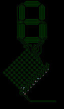
Quality desires to be better – another reason I wanted to remake it. It seems like every cell of WireWorld structure corresponds to exactly one pixel in that frame. This is not surprising – person who generated it probably chosen this as a simplest setting to make the .GIF. Now let see how many colors in that image – a good guess is 4 because of the rules of the WireWorld – colors are background, wires, and heads and tails of electrons. Well good guess:


But these are RGB colors. I need data presented by a matrix with elements given by integers from 0 to 3. So which color corresponds to which integer? Careful examination of the image makes things clear:


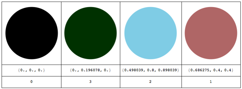
Now the simple step of constructing the WireWorld structure out of Wikipedia image:And with just a few lines of code we can light it up – what a marvelous pixel perfect spectacle!


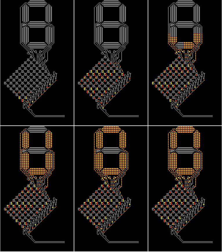
I used built in function CellularAutomaton that made thing so easy and adopted a snippet of code from the Rosetta Code page (btw Mathematica code there is the shortest I think). 

Now have you ever thought about random circuits? Why would you think about them? Well because browsing random circuits you can discover interesting elements that you would not know exist. This is sometimes called “exploring the computational universe” abut which you can find out in the New Kind of Science book or learn hands on in the Wolfram Science Summer School.

Here I build a random circuit using another delightful Elementary Cellular Automaton Rule 54. It has a few cool properties, for example being a candidate for computational universality. But we interested in its ability to produce wiry patterns of complex shapes suitable for running WireWorld on them. These are difference patterns which are sort of analogy of Butterfly Effect in discrite world of bytes. The question we are asking here is not “if we get a hurricane if butterfly had flapped its wings earlier”, but if we get something interesting by flipping a single bit in a massive evolution in discrete space. Here is a function that builds a random circuit of difference pattern of Rule 54 and then runs WireWorld on it.Here are a few samples:


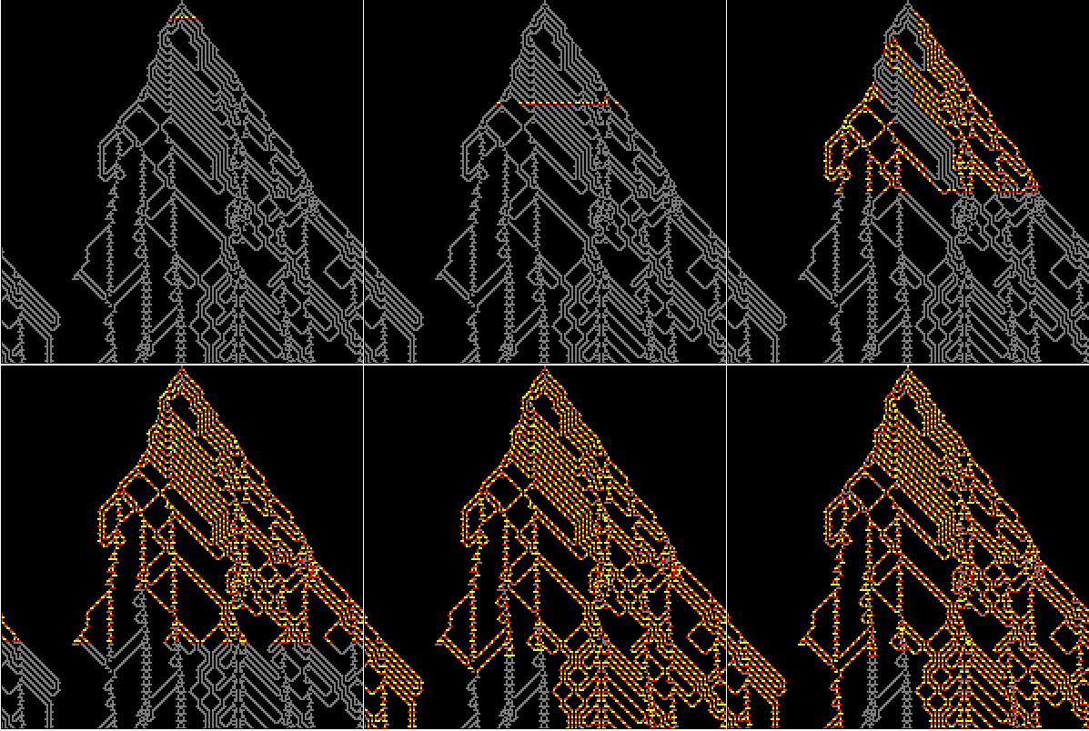
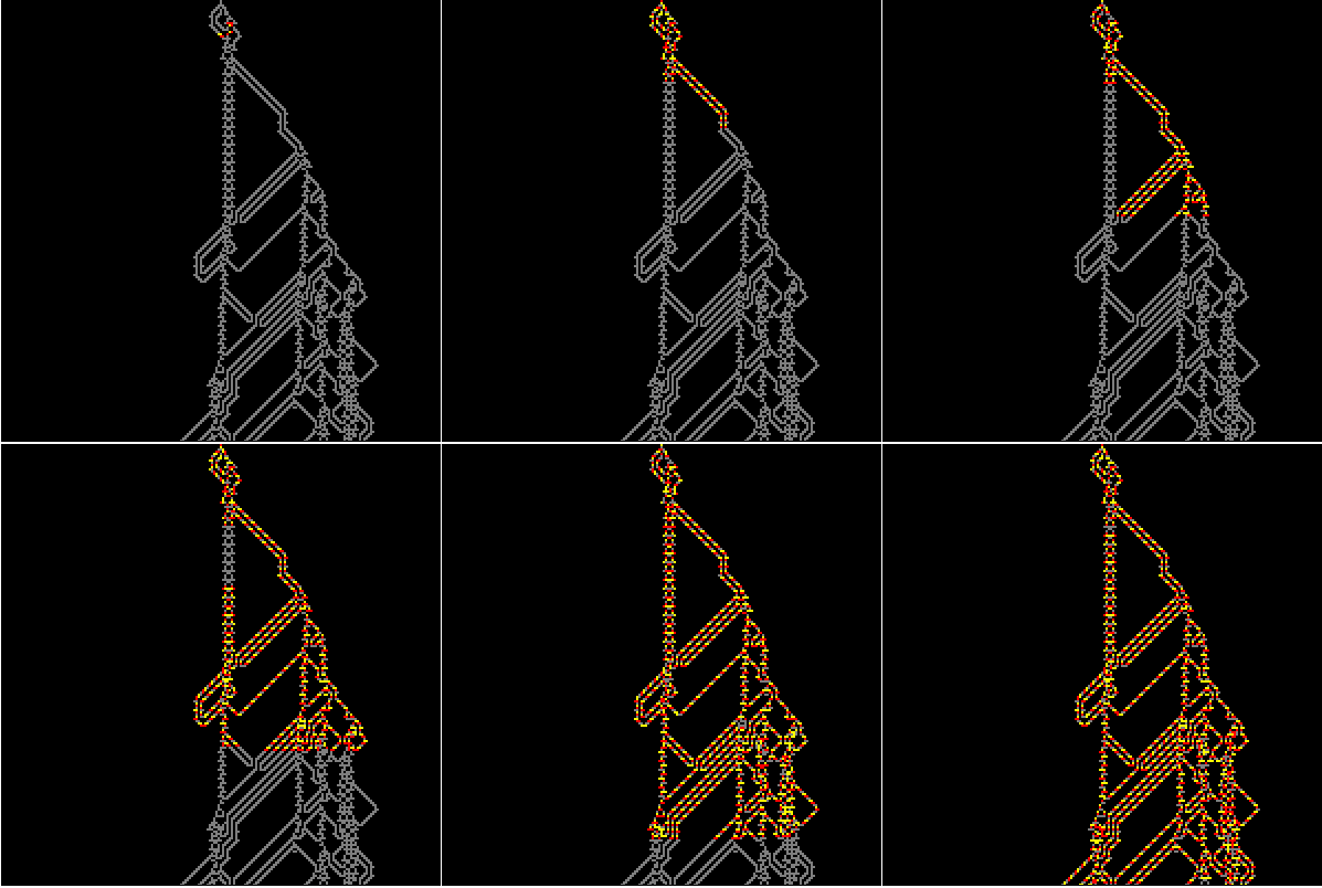
What can we immediately notice? A single electron can run as it is, alone, until it hit a structure that can generate more electrons. Another thing – there are structures that do not conduct electrons in one direction, but do so in the opposite one – they are called diodes.

And of course, as soon as I finished all this, someone let me know that the data for largest circuit - The Wireworld Computer – is available on this webpage. To see it running we first need to import data. The data are in archived ZIP file which Mathematica understands perfectly. Let's see what is inside the ZIP file:Let's digg that out:Now the file is basically text and we need to do some conversion to numerical matrix. 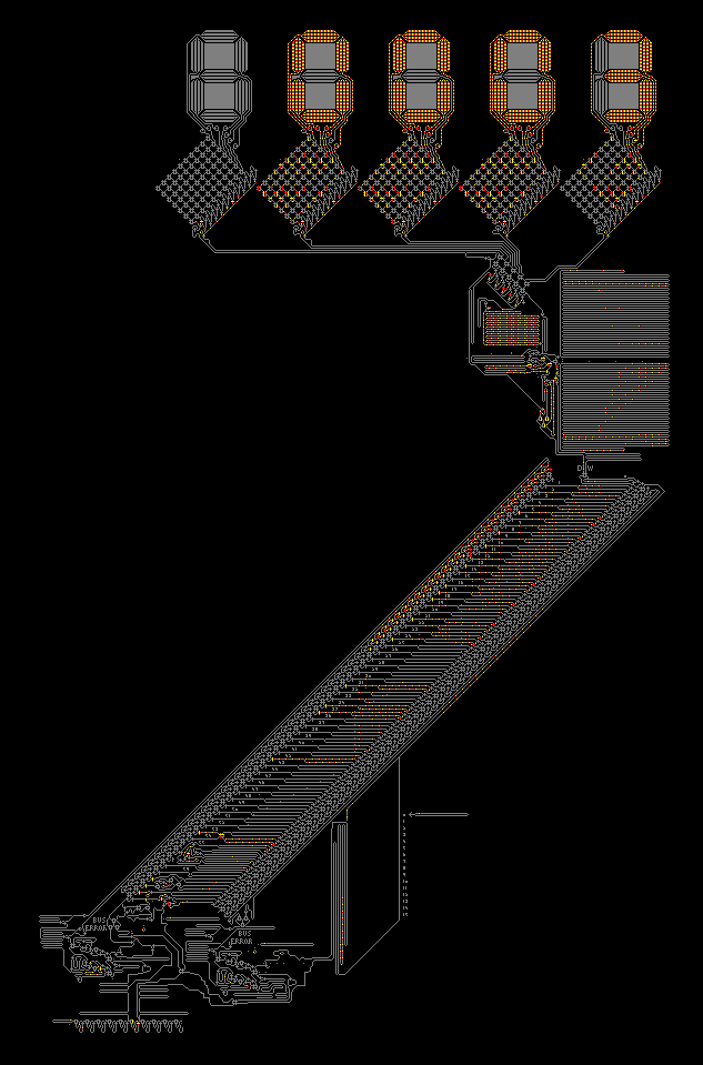Symbol “@” is the head, “~” is the tail, and “#” is the wire:Now we can run this awe-inspiring structure as we did before: 


To discover more things check out a great recently published demonstration that inspired me to check this all out:

WireWorld Gates and Gadgets