Introduction
The goal of this project is to analyze property descriptions of real estate and identify words that positively or negatively affected the success of a sale. Success of a sale is measured as the percent difference between the listing and selling prices of the property. Data for this project were gathered from MLS through redfin.com and analyzed using Wolfram Mathematica's text analysis functions and neural nets from the Wolfram Neural Net Repository. Through a TF-IDF analysis of the data, clustering functions, and an analysis of frequently used words, correlations between word content and sale success were identified.
This project focussed on properties sold in the Boston area from April to June of 2018. Future research would include a much broader set of data to see if the trends identified in this analysis hold outside of the city of Boston and if more trends can be identified. Though the description of a property is just one of many factors that affect the sale of a home, this project aims to understand the potential importance of word choice in the industry.
TF-IDF Analysis
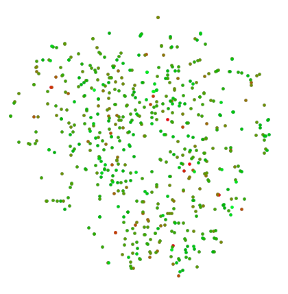
Through a TF-IDF analysis of each listing, the words that were most unique to each listing were identified. A neural net from the Wolfram Neural Net Repository was used to make a feature space plots of the words shown below, where similar words are shown closer together. Each point, representing a word, is colored on a scale of red to green by score and then rank, red representing an unsuccessful sale and green representing a successful sale.
A list of house listings, each in the form {house description (string), percent difference between listing and selling price of the house (number)}:
data = Get["data.mx"];
A list of the house descriptions:
corpus = data[[All, 1]];
The corpus without stopwords or numerical values:
tokenizedCorpus = Select[TextWords@ToLowerCase@DeleteStopwords@#,
    !StringContainsQ[#, {"0", "1", "2", "3", "4", "5", "6", "7", "8", "9"}] &] & /@ corpus;
A neural net from the Wolfram Neural Net Repository for feature extraction of words:
glove = NetModel["GloVe 100-Dimensional Word Vectors Trained on Wikipedia and Gigaword 5 Data"];
Functions to determine term frequency and inverse document frequency of each word. The product of these two results is a word's TF-IDF score:
tf[word_String, tokenizedText_] := N[Count[tokenizedText,word] / Length[tokenizedText]]

idf[word_, tokenizedCorpus_] := N @ Log[ 10, Length[tokenizedCorpus] / Count[tokenizedCorpus, l_List /; MemberQ[l ,word]] ]
A list of associations, one for each listing, in which each word in a listing is associated with its TF-IDF score:
wordScores=Table[AssociationMap[tf[#,tokenizedCorpus[[n]]]*idf[#, tokenizedCorpus]&,DeleteDuplicates@tokenizedCorpus[[n]]],
    {n,Length[tokenizedCorpus]}];
The top five words, based of TF-IDF score, of each listing:
wordScoresTopFive = Take[Sort[#, Greater], 5] & /@ wordScores;
A list of top words from every listing in the form {word, score of listing} with the scores of duplicate words averaged:
allTopWords = Flatten[Table[{#, Last[data[[n]]]} & /@ Keys[wordScoresTopFive[[n]]], {n, Length[wordScoresTopFive]}], 1];
allTopWords = SortBy[{First[First[#]], Mean[Last /@ #]} & /@ GatherBy[allTopWords, First], Last];
A list of words whose listing has a negative score:
negativeWords = Select[allTopWords, Last[#] < 0 &];
Negative scores rescaled between 0 and 0.5 which will correspond to different shades of red:
rescaledNegativeScores = Rescale[negativeWords[[All, 2]], MinMax[negativeWords[[All, 2]]], {0, 0.5}];
A list of words whose listing has a score of 0:
neutralWords = Select[allTopWords, Last[#] == 0 &];
Words with neural scores assigned a score of 0.5 which will correspond to a mix of red and green:
rescaledNeutralScores = Table[0.5, Length[neutralWords]];
A list of words whose listing has a positive score:
positiveWords = Select[allTopWords, Last[#] > 0 &];
Positive scores rescaled between 0.5 and 1 which will correspond to different shades of green:
rescaledPositiveScores = Rescale[positiveWords[[All, 2]], MinMax[positiveWords[[All, 2]]], {0.5, 1}];
The scores of all top words rescaled to values between 0 and 1:
rescaledScores = Join[rescaledNegativeScores, rescaledNeutralScores, rescaledPositiveScores];
A list of each top word in the form {word, rescaled score}:
rescaledWords = Transpose[{allTopWords[[All, 1]], rescaledScores}];
A feature space plot that used a neural net to map each word. The color of each word corresponds to its success:
FeatureSpacePlot[Style[First[#], RGBColor[1 - Last[#], Last[#], 0]] & /@ rescaledWords, FeatureExtractor -> glove,
    LabelingFunction -> Tooltip, ImageSize -> Large, PlotStyle -> Directive[PointSize[Medium]]]
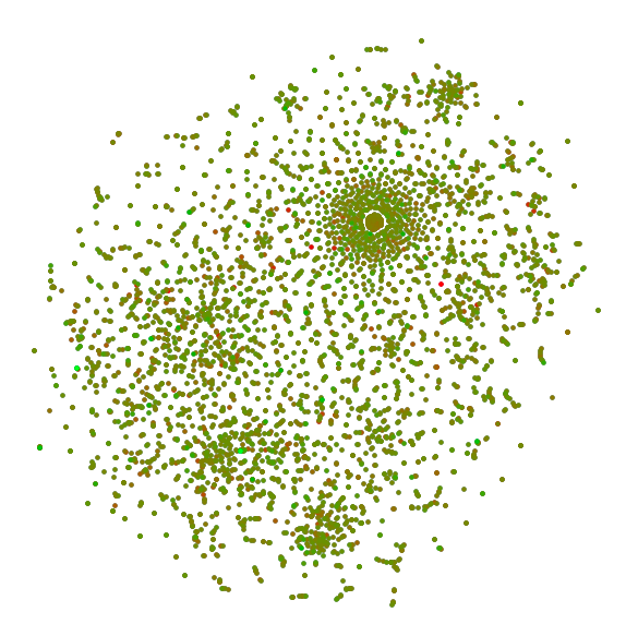
The ranks of all top words, from lowest to highest TF-IDF score, scaled from 0 to 1:
ranks = Rescale[Range[Length[allTopWords]], MinMax[Range[Length[allTopWords]]], {0, 1}] // N;
A list of each top word in the form {word, rank}:
rankedWords = Transpose[{allTopWords[[All, 1]], ranks}];
A feature space plot that used a neural net to map each word. The color of each word corresponds to its success:
FeatureSpacePlot[Style[First[#], RGBColor[1 - Last[#], Last[#], 0]] & /@ rankedWords, FeatureExtractor -> glove,
    LabelingFunction -> Tooltip, ImageSize -> Large, PlotStyle -> Directive[PointSize[Medium]]]
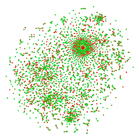
This analysis revealed several trends. First, misspelled words, words with slashes or hyphens, most abbreviations, and words associated with measurement, water, and public transportation were correlated to unsuccessful sales. Additionally, words associated with locations in a home (bedroom, closet, floor, room, patio, parlor, basement, attic, porch, atrium, yard, foyer, courtyard, etc.) as well as words referring to time (days of the week, months, seasons, etc.) were correlated to successful sales. The mixture of red and green dots throughout the graph shows that words with similar meanings did differently. For example, the words "wifi", "gracious", and "fantastic" occurred in successful listings, while the words "wireless", "gorgeous", and "awesome" occurred in unsuccessful listings. This indicates that word choice is extremely important though more data are needed to further explore this trend.
Additionally, several trends were specific to Boston. Many listings, both successful and unsuccessful, mentioned specific locations or monuments in the city (Kendall Square, Fenway Park, Copley, Cambridge, etc.), words that would not be relevant in a large data set with areas outside of Boston included. Words associated with water (wharf, harbor, waterfront, port, seafront, etc.) and words associated with public transportation (metro, tstop, busline, etc.) did very badly, something that may or may not be specific to Boston.
Clustering
Using the words with the highest TF-IDF scores, clustering functions were used along with a neural net to divide words into sets based on similarity, excluding terms that were not real words such as names and places. This allowed further analysis of trends identified in the feature space plot, particularly which categories of words were positive or negative, and which categories had words that had a range of success. Below is a feature space plot of words colored according to cluster:
The multidimensional embeddings of each word:
wordEmbeddings = glove[allTopWords[[All, 1]]];
An association of embedding of word to word for each word:
embeddingsToWords = AssociationThread[wordEmbeddings, allTopWords[[All, 1]]];
Embeddings divided into clusters:
embeddingClusters = FindClusters[wordEmbeddings, Method -> "GaussianMixture"];
The same clusters with words instead of embeddings:
wordClusters = Map[embeddingsToWords, embeddingClusters, {2}];
Colors to represent each cluster:
colors = Table[RandomColor[], Length[embeddingClusters]];
An association of embedding to color of cluster the embedding belongs to. Terms that are not real words, such as places and names, have been excluded:
coloredByCluster = Flatten[Table[{#, colors[[n]]} & /@ embeddingClusters[[n]], {n, Length[embeddingClusters]}], 1];
coloredByCluster = Select[coloredByCluster, First[#] != glove["notaword"] &];
A feature space plot of all word embeddings. Each dot represents a word and each color represents a cluster. Terms that are not real words, such as places and names, have been excluded:
FeatureSpacePlot[Style[embeddingsToWords[First[#]], Last[#]] & /@ coloredByCluster, FeatureExtractor -> glove,
    LabelingFunction -> Tooltip, ImageSize -> Large, PlotStyle -> Directive[PointSize[Medium]]]
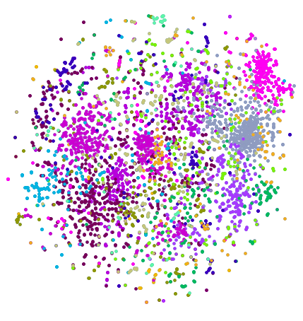
These clusters allow different categories and types of words to be compared. The average score of each cluster is calculated and histograms of the scores of each cluster are shown below. This information shows that words from any given category had a range of success, confirming that similar words performed differently, just as the feature space plot showed.
An association of words and their scores:
wordsToScores = AssociationThread[First /@ allTopWords, Last /@ allTopWords];
Clusters of words excluding terms that are not words:
wordClustersWordsOnly = Map[embeddingsToWords,
    Map[Function[cluster, Select[cluster, # != glove["notaword"] &]],embeddingClusters], {2}];
Clusters of the scores of words that belong to each cluster:
scoreClusters = Map[wordsToScores, wordClustersWordsOnly, {2}];
The average performance of the words in each cluster relative to the average performance of all words:
means = Mean /@ scoreClusters - Mean[Flatten[scoreClusters]]

{0.0842496, -1.81491, -0.0842654, -0.383492, -0.312529, 0.052031, -0.148875, 0.10506, 0.535048, 0.551549, 0.396386,
 -0.0538008, -0.0692717, -0.0364944, 0.0809207}
Histograms of the scores of the words in each cluster:
histograms = Histogram /@ scoreClusters
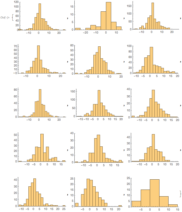
The second histogram had the lowest average score, meaning that the words in this category were unsuccessful. These were the following words, from lowest to highest score, of the words in that cluster which are all associated with measurement:
wordClustersWordsOnly[[2]]

{"acres", "land", "fifty", "half", "vacant", "irrigated", "sixty", "tons", "remaining", "meter", "sq", "radius", "compared",
 "occupying", "mile", "total", "meters", "ft", "reclaimed", "allocated", "occupied", "thirty", "width", "m", "acre",
 "square", "yards", "approx", "miles", "completed", "height", "approximately", "fell", "feet", "million", "occupies",
 "foot", "½", "units", "length", "quarters", "seats", "mi", "soldiers"}
Clustering allowed a closer examination of the data, allowing trends discovered by a TF-IDF analysis and feature space plots to become clearer. Additionally, clustering allows room for future exploration of the data. In the future, individual clusters can be analyzed, clusters can be compared, and different clustering methods could be applied.
Frequency Analysis
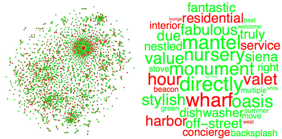
In addition to a TF-IDF analysis of the data, words occurring in at least 1% of listings were identified and scored according to the average success of the listings in which a word was used. These scores allowed words correlated with successful and unsuccessful sales to be identified. This analysis revealed that successful listings shared many similar words while unsuccessful listings had very little overlap. Lists of the most and least successful words are shown below along with a word cloud to visualize the data:
A list of house listings, each in the form {house description (string), percent difference between listing and selling price of the house (number)}:
data = Get["data.mx"];
The house descriptions without stopwords or numerical values:
tokenizedData = Transpose[{Select[TextWords@ ToLowerCase@DeleteStopwords@First[#],
    !StringContainsQ[#, {"0", "1", "2", "3", "4", "5", "6", "7", "8", "9"}] &] & /@ data, data[[All, 2]]}];
A neural net from the Wolfram Neural Net Repository for feature extraction of words:
glove = NetModel["GloVe 100-Dimensional Word Vectors Trained on Wikipedia and Gigaword 5 Data"];
A list of words from every listing in the form {word, score of listing}:
allWords = Flatten[Transpose[{First[#], Table[Last[#], Length[First[#]]]}] & /@ tokenizedData, 1];
A list of words that occur in more than 1% of listings, scored according to the average success of the listings in which a word was used:
mostFrequentWords = Select[GatherBy[allWords, First], Length[#] > 30 &];
mostFrequentWords = SortBy[{First[First[#]], Mean[Last /@ #]} & /@ mostFrequentWords, Last];
A list of frequent words whose listing has a negative score:
negativeWords = Select[mostFrequentWords, Last[#] < 0 &];
Negative scores rescaled between 0 and 0.5 which will correspond to different shades of red:
rescaledNegativeScores = Rescale[negativeWords[[All, 2]], MinMax[negativeWords[[All, 2]]], {0, 0.5}];
A list of frequent words whose listing has a positive score:
positiveWords = Select[mostFrequentWords, Last[#] > 0 &];
Positive scores rescaled between 0.5 and 1 which will correspond to different shades of green:
rescaledPositiveScores = Rescale[positiveWords[[All, 2]], MinMax[positiveWords[[All, 2]]], {0.5, 1}];
The scores of all the most frequent words rescaled to values between 0 and 1:
rescaledScores = Join[rescaledNegativeScores, rescaledPositiveScores];
A list of each top word in the form {word, rescaled score}:
rescaledWords = Transpose[{mostFrequentWords[[All, 1]], rescaledScores}];
A feature space plot that used a neural net to map each word. The color of each word corresponds to its success:
FeatureSpacePlot[Style[First[#], RGBColor[1 - Last[#], Last[#], 0]] & /@ rescaledWords, FeatureExtractor -> glove,
    LabelingFunction -> Tooltip, ImageSize -> Medium, PlotStyle -> Directive[PointSize[Medium]]]
The words that were unsuccessful in order from most unsuccessful to least unsuccessful:
mostNegativeWords = First /@ Select[mostFrequentWords, Last[#] < -1 &]

{"wharf", "residents", "services", "hour", "valet", "fireplaces", "harbor", "residential", "service", "month",
 "concierge", "interior", "converted", "years", "beacon", "lot", "sf", "west", "lounge", "club"}
The words that were successful in order from least successful to most successful:
mostPositiveWords = First /@ Select[mostFrequentWords, Last[#] > 1 &];
Some of the most successful words from least successful to most successful:
mostPositiveWords[[325 ;; 388]]

{"sun-filled", "stained", "tile", "doors", "front", "seating", "gem", "white", "urban", "wonderful", "sale", "welcome",
 "best", "wide", "summer", "green", "multiple", "in-unit", "move", "sunday", "stove", "cambridge", "recessed",
 "backsplash", "exposure", "abundant", "savin", "landscaped", "tree-lined", "right", "rear", "lines", "nestled",
 "porch", "fenced", "dishwasher", "fantastic", "truly", "off-street", "siena", "leading", "due", "love", "saturday",
 "fabulous", "sink", "stylish", "seller", "charming", "value", "fenway", "showings", "pm", "oasis", "monument",
 "nursery", "monday", "april", "houses", "march", "mantel", "tuesday", "directly", "copley"}
A selection of some of the most influential words:
wordCloudWords = Join[mostNegativeWords, mostPositiveWords[[325 ;; 388]]];
Each word and a weight that will be used to size the word in a word cloud:
negativeAssoc = AssociationThread[mostNegativeWords, Reverse[Range[3, 60, 3]]];
positiveAssoc = AssociationThread[mostPositiveWords[[325 ;; 388]], Range[64]];
weights = Join[Values[negativeAssoc], Values[positiveAssoc]];
wordToWeight = AssociationThread[wordCloudWords, weights];
The color of each word in the word cloud, red for negative words and green for positive words:
colors = Join[Table[Red, Length[mostNegativeWords]], Table[Green, Length[mostPositiveWords[[325 ;; 388]]]]];
wordToColor = AssociationThread[wordCloudWords, colors];
A word cloud of some of the most frequent words and their relative success. Unsuccessful words are shown in red and successful words in green. The larger the word, the greater its impact:
WordCloud[{Style[#, wordToColor[#]], wordToWeight[#]} & /@ allWords]
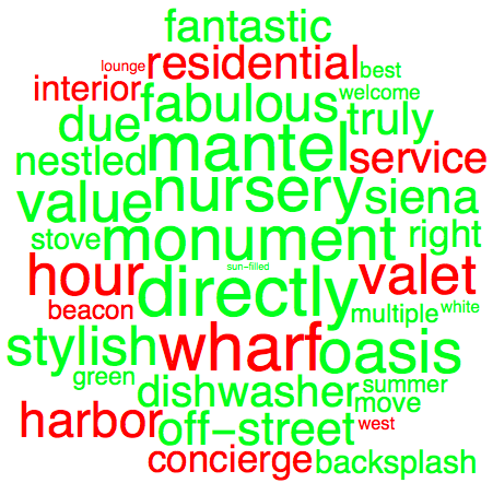
An analysis of the most frequently used words provided a different perspective of the data. Through this analysis, words that were widely successful or unsuccessful could be identified and their relative impact could be determined.
Summary of Results
A TF-IDF analysis of the data found that words with slashes or hyphens, misspelled words, most abbreviations, and words associated with measurement, water, and public transportation were unsuccessful while words associated with time and locations in a house were successful. A feature space plot of all the words, mapped by a neural net, showed that often similar words performed very differently; for example, the words "wifi", "gracious", and "fantastic" did well while the words "wireless", "gorgeous", and "awesome" did poorly. Though more data are needed to confirm this trend, these results indicate that word choice may be extremely important.
Clustering functions along with a neural net were used to map and divide words based on similarity. This categorization allowed a much closer examination of the data and confirmed trends found in the TF-IDF analysis. Through a feature space plot of the clusters, the average score of the words in each cluster, and histograms of the scores of the words in each cluster, clusters could be analyzed individually and compared to each other, providing a deeper exploration of the data.
In addition to a TF-IDF analysis and the use of clustering, the most frequent words in all listings were identified. There were more successful words than unsuccessful indicating that successful listings shared many similar words while unsuccessful listings had very little overlap. The relative impact of each of these words was identified and a word cloud was created to visualize this information.
Through a TF-IDF analysis, clustering, and an analysis of the most frequent words, this project successfully identified several trends between word content and sale success in home listings.
Future Directions
This analysis used data from a three month period in Boston. Future research could examine different cities, rural locations, and a timeframe of more than three months. Additionally, the description of a home is only one of many factors in the success of a sale. Future work could identify and examine the many factors that affect the success of a sale and the importance of each factor.
Code and Data Files
https://github.com/nd-2567/WSS2018
Data Sources
https://www.redfin.com/
http://www.mls.com/
Background Information and References
https://en.wikipedia.org/wiki/Tf%E2%80%93idf
https://resources.wolframcloud.com/NeuralNetRepository/
Author Contact Information
dadanatasha@gmail.com
 Attachments:


