The goal of this work is to train a convolution neural network to solve partial differential equations (PDEs) more efficiently than the existing numerical methods. The proposed method can do faster estimations, and solve for conditions where other estimations do not converge.
Background
PDE's are pervasive in the field of physics, mathematics, and chemical science. Even if there are many ways of estimating the solution of these equations, they are computationally very expensive, and also fail to converge at certain conditions. In contrast, Neural Networks are also universal function approximators, therefore, they can be applied to more "classical" mathematical problems such as PDEs.
Methodology
The approach is to design and train a convolution-based neural network using the density plot results from the inbuilt finite element solver in wolfram script, and predict the values for different regions. Then the work is expanded to changing coefficients in the Fick' s law of diffusion to validate performance during the time-dependent non-linear behaviour of PDEs.
Equation 1: Modified Fick's law of diffusion
The first modified equation varies in terms of x and y spatial coordinates as shown:
$$\frac{\partial \varphi (x,y)}{\partial y}=a\frac{\partial ^2\varphi (x,y)}{\partial x^2}-b$$
The training sets of this model were created using convex-hull mesh, for a variety of randomized shapes. The code could be found below in the embedded notebook. The model was trained using a 7 layer Network, which was used to train colour images, then the model was increased to 11 and finally 21 layers. To keep the training time lesser with an increase in the overall size of the trained net, a switch to black and white images was done with grid sizes of {120*120} and {210,210}. The results have been shown in the following figure to compare the three nets, with their percentage accuracy and converging time. 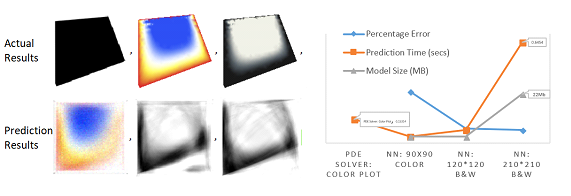
The error rate of the three models kept decreasing from 33% to 9% and finally 8%, with an exponential increase in the model size: 3 MBs in the initial cases to 25 Mb for the {220*220} images. To the dismay, however, the convergence time required by the final model was even 4 times higher than the actual PDE solver, but we will see later that as the complexity of PDE's increase, the neural networks do a significantly better job.
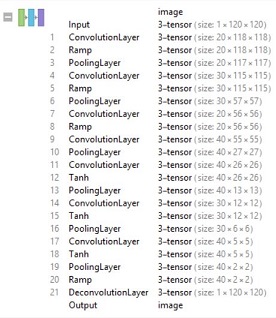
A snapshot of the final network can be seen in the next figure for recreating the same results, and the code notebook for generating the data has been embedded at the end.
Equation 2:Time-varying non-linear PDEs: Fick's first law of diffusion
Further, the finite element solutions actual Fick's law of diffusion (only in x-direction) were used to train the neural networks for multiple values of the diffusion coefficient.
$$\frac{\partial \varphi (x,t)}{\partial t}=c\frac{\partial ^2\varphi (x,t)}{\partial x^2}$$
The same layers of neural network were used to train this equation. However, the input for this network were scalar quantities of varying coefficients of diffusion, i.e c. Hence, a constant matrix of 20*20 was used as an input to the network. The code snippet for doing the same is as follows:
sol[c_, x0_] :=
NDSolve[{D[u[t, x], t] == c D[u[t, x], x, x], u[0, x] == 0,
u[t, 1] == 0.1}, u, {t, 0, 10}, {x, 0, 1}]
raw[c_] := Image[ConstantArray[(c/50), {20, 20}]]
    result[c_] :=
     ColorConvert[
      DensityPlot[Evaluate[u[t, x] /. sol[c, 1]], {t, 0, 10}, {x, 0, 1},
       PlotRange -> All, ColorFunctionScaling -> False,
       ColorFunction -> ColorData[{"GrayTones", {-0.05, 0.05}}],
       BoundaryStyle -> None, Frame -> False], GrayLevel]

        (*creating the data*)
        data = {};
        c = 0.1;
        Do[data = AppendTo[data, raw[c] -> result[c]];
         c = Round[RandomReal[{0.01,
            2}],0.01],(* random sampling to aid training of the net*)
         {5000}]
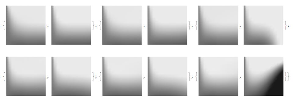
The results generated in the training show a varying level of accuracy owing to the non-linear behaviour of the PDEs. Also, with an increase in training time, it was observed that the network was getting increasingly better at predicting the non-linear behaviour, as can be observed in the following results [Predictions->Actual results] with a training data of 5000 sets between the diffusion coefficient randomly distributed between {0.01 to 2}. The plots made for these results represent a plot of x co-ordinates{0,1} varying vs time{0,10}.
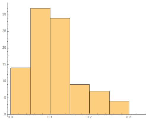
The average error of the results come to be around 8.5%, with some samples as accurate as 98%, to an occasional inaccuracy of 30%. The histogram of the error distribution can be seen in the following figure. The x-axis represents the error in the scale of 1, and y is the distribution.
The average recorded absolute speed for prediction using the neural networks was found to be at least 6 times faster for a 1D Fick's law. This provided promise than neural networks could be a great tool in reducing the complexity of one of the major complexities of mathematics.
Conclusions and Future work
Neural networks are indeed a great way to predict the behaviour of partial differential equations. It would be great to explore the neural nets for architectures better at learning non-linear behaviour. Also, increasing the dimensions and the complexity of the nets could find the neural nets even more efficient as compared to the current estimation methods.


