Rooftop Recognition for Solar Energy Potential

The aim of this project is to detect the rooftop of buildings to determine the available area at different locations and to identify the most suitable ones for solar energy application such as solar PV using Neural Networks and satellite imagery.

Github link for files and notebooks: https://github.com/enricocg/Project

The Dataset

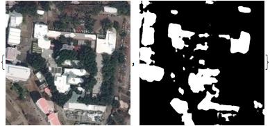
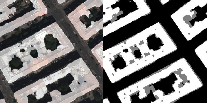
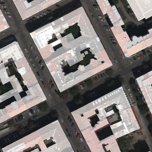
The Inria Aerial Image Labeling addresses a core topic in remote sensing: the automatic pixelwise labeling of aerial imagery. Dataset features:

• Coverage of 810 km (405 km for training and 405 km for testing)
• Aerial orthorectified color imagery with a spatial resolution of 0.3 m
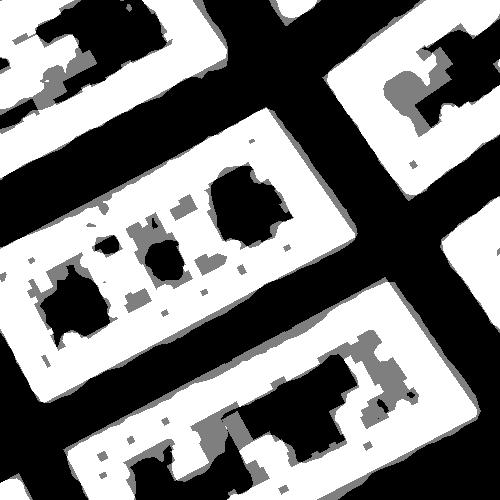
• Ground truth data for two semantic classes : building and not building (publicly disclosed only for the training subset)

https : // project.inria.fr/aerialimagelabeling/

Select the images for the input and those for the results:

trainFilesInput = 
Select[FileNames[
"image/*.tif"], ! StringMatchQ[#, ___ ~~ "._" ~~ ___] &];
trainFilesResult = 
StringReplace[#, "image/" -> "mask/"] & /@ trainFilesInput;

Import an image to test:

imgInput = Import[trainFilesInput[[1]]];
imgResult = Import[trainFilesResult[[1]]];

Partition of the images in 100 from a 5000x5000 to images 500x500 :

splicesInput = Join @@ ImagePartition[imgInput, 500];
splicesResults = Join @@ ImagePartition[imgResult, 500];

Assemble Images

Assemble images in sets of ten to verify:

assambleImage = ImageAssemble[splicesInput[[41 ;; 50]]]

Assemble mask images in sets of ten to verify:

assambleMask = 
 ImageAssemble[
  Image /@ Round[ImageData /@ splicesResults[[41 ;; 50]]]]

Compose

Compose the images to verify image matching:

ImageCompose[assambleImage, {assambleMask, 0.5}]

rand = RandomInteger[{1, 100}];
ImageCompose[splicesInput[[rand]], {splicesResults[[rand]], 0.5}]

Association

mxTrain = Thread[splicesInput -> splicesResults];

ImageCompose[Keys[mxTrain[[rand]]], {Values[mxTrain[[rand]]], 0.4}]

Export the MX file

Export["File.mx", mxTrain]

Export

mxFileCreator

The first approach to organize the data was to make MX files, one per image, each file contain the 100 images with their respective mask. In order to do that a function mxFileCreator was build.

Function that creates a MX file per each 5000x5000 image:

mxFileCreator[trainFilesInput_,trainFilesResult_,i_]:=Block[
    {Flag,imgInput,imgResult,splicesInput,splicesResults,mxTrain},

    Flag=TextString[i];

    imgInput=Import[trainFilesInput];
    imgResult=Import[trainFilesResult];

    splicesInput=Join@@ImagePartition[imgInput,500];
    splicesResults=Round[ImageData/@(Join@@ImagePartition[imgResult,500])];

    mxTrain=Thread[splicesInput-> splicesResults];

    Export["MXFiles/File"<>Flag<>".mx",mxTrain]
]

Test the function

mxFileCreator[trainFilesInput[[1]], trainFilesResult[[1]], 1]
"MXFiles/File1.mx"

file = Import["MXFiles/File1.mx"];
file[[RandomInteger[{1, 100}]]]

ImageCompose[Keys[file[[rand]]], {Image[Values[file[[rand]]]], 0.5}]

To Map all the images and convert them into association in a MX files :

MapIndexed[mxFileCreator[#[[1]], #[[2]], Echo[#2[[1]]]] &, 
 Transpose[{trainFilesInput, trainFilesResult}]]

The net

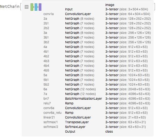
The net selected for this project was at Wolfram Neural Net Repository for Semantic Segmentation. Released in 2016 by the University of Adelaide, Ademxapp Model A1 Trained on PASCAL VOC2012 and MS-COCO Data was modify to identify two classes instead of 21.

Take the net model for Semantic Segmentation from the repositories:

netModel = 
 NetModel["Ademxapp Model A1 Trained on PASCAL VOC2012 and MS-COCO \
Data"]

Net surgery

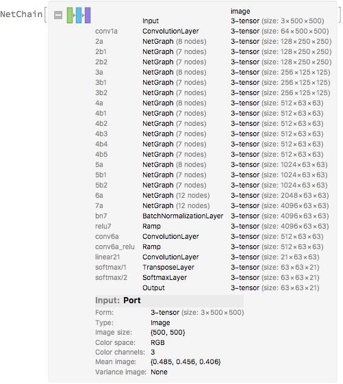
Modify the Input for the size of the images

netModel500 = NetReplacePart[netModel, "Input" -> NetEncoder[{"Image", {500, 500}, "MeanImage" -> {0.485, 0.456, 0.406}}] ]

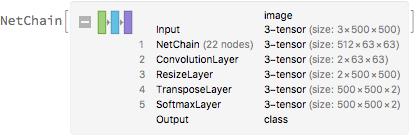
Resize the layer

Drop the last three layer to modify the net:

firstPartNet = NetDrop[netModel500, -3]

Convolution layer

Add a convolution layer to have two outputs:

convLayer=NetChain[{firstPartNet, ConvolutionLayer[2, {3, 3}, "Stride" -> {1, 1}, "PaddingSize" -> {12, 12}, "Dilation" -> {12, 12}], ResizeLayer[{500, 500}]}];

Take the last two layers from the one with the new encoder:

lastPartNet = NetReplacePart[NetTake[netModel500, -2], "Input" -> Automatic]

SoftmaxLayer

Append the last layers and Softmax Layer with a net decoder of classes:

finalNet = NetAppend[convLayer, {lastPartNet[[1]], SoftmaxLayer[]}, "Output" -> NetDecoder[{"Class", {0, 1}, "InputDepth" -> 3}]]

Initialize the net

Initialize the final net to check for errors:

iniFinalNet = NetInitialize[finalNet]

Net to train

Loss Function

Connect the final net to a loss function:

LossNet = NetGraph[<|"eval" -> finalNet, "loss" -> CrossEntropyLossLayer["Index"]|>, {"eval" -> "loss"} ]

Initialize the LossNet:

iniLossNet = NetInitialize[LossNet]

Export the complete net for training:

Export["iniLossNet.wlnet", iniLossNet]

Generator function

Reduce Dataset Size

From the MX files created in section. Set the file path for the MX files:

path = "MXFiles/";
mxFiles = FileNames[path <> "*.mx"];
RandomSample[mxFiles, 1][[1]]

Binary Files

Binary files are a way to reduce of the size while importing the train set. Once the files are binarize the file size reduces and ones read in can be deserialize. At the same time TIF images were converted to JPG to remove unnecessary information while reducing size.

Binary write:

binaryWrite[file_,expr_]:=With[{bytes=BinaryWrite[file,BinarySerialize[expr]]},
    Close[file]; bytes]

Function to convert TIF images to JPG and matrix to Binary:

importAndReExport[path_,folder_]:=Block[{imported,imgs,masks,hashes},
    imported=Import[path];
    imgs=imported[[All,1]];
    masks=imported[[All,2]];
    hashes=Hash/@imgs;

    Print[MapThread[Export[folder<>"/"<>ToString[#1]<>".jpg",#2]&,{hashes,imgs}];//AbsoluteTiming];
    Print[MapThread[binaryWrite[folder<>"/"<>ToString[#1]<>".bin",#2]&,{hashes,masks}];//AbsoluteTiming];

    Clear[imported,imgs,masks,hashes]
]

Take each MX file and create the correspondent JPG and BIN file :

Table[importAndReExport[mxFiles[[i]], "binFiles"], {i, 1, Length[mxFiles], 1}]

Binary Read

Read the binary file and Deserialize the file:

BinaryDeserialize[ReadByteArray["/Users/enricocastro/Documents/GitHub/Project/binFiles/\74004748475675200.bin"]] // Dimensions

Training Out of Core

Partitional Function

Data from MX files

Take the name of the JPG and BIN files:

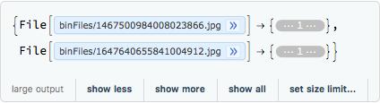
trainingDataSet = {FileNames["binFiles/*.jpg"], FileNames["binFiles/*.bin"]};

Set the data to train:

imageDataSet = Table[File[trainingDataSet[[1, i]]], {i, 10}];
maskDataSet = Table[ReadByteArray[trainingDataSet[[2, i]]], {i, 10}];

Associate the image with his respective mask and take a random sample:

data = RandomSample@Thread[imageDataSet -> maskDataSet];
data[[2]]

Generator

In order to train the net with a big amount of data a generator function was created. The generator function load a single batch of data from an external source to train each time. NetTrain[net, f, [Ellipsis]] calls f at each training batch iteration, thus only keeping a single batch of training data in memory. The function can depend on the batch size, which can be set or set automatic by the computer, the absolute batch that is the number of batches load during the training and the round.

partGenerator associate and load a batch of size BatchSize into the net training. In order to do so it takes partitions of the whole dataset in batches of size BatchSize and load the element of this partition taking the module of the AbsoluteBatch. The function also adds one to the mask matrix to get the right values for the net:

partGenerator=Function[Block[{batch,dataSet,batchData},
    If[!ValueQ[partitionedData],partitionedData=Partition[Range[Length[data]],#BatchSize,#BatchSize,1]];
    Print[Association@Thread[Keys[#]->Values[#]]];
    batch=Mod[#AbsoluteBatch,Floor[Length@data/#BatchSize]];
    batchData=data[[partitionedData[[Echo@(batch+1)]]]];

    Thread[Keys[batchData]->1+BinaryDeserialize/@Values[batchData]]
    (*<|"Input"\[Rule]Keys[batchData],"Target"\[Rule]BinaryDeserialize/@Values[batchData]|>*)
    ]
];

Test of partGenerator

partGeneratorData = 
 partGenerator[<|"BatchSize" -> 2, "Round" -> 0, 
   "AbsoluteBatch" -> 1|>]

Train test

Before training for a lot of data is always good to try first with a small set. Clear partitionedData for different batch sizes:

ClearAll[partitionedData];

iniLossNet = Import["iniLossNet.wlnet"]

Set the checkpoint directory:

checkpointDir = "checkpoint"

Net training with partGenerator:

iniLossTrainNet = NetTrain[iniLossNet, {partGenerator, "RoundLength" -> 3}, All, MaxTrainingRounds -> 3, TrainingProgressCheckpointing -> {"Directory", checkpointDir}]

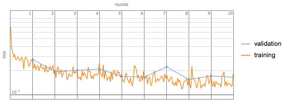
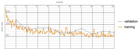
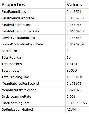
Trained Net

Once trained one can look at the relevant information of the training process. Import the trained net as an object:

Encoder & Decoder

Set the encoders and decoders for further tests. Set the encoder for image size 500x500 and a MeanImage:

enc = NetEncoder[{"Image", {500, 500}, "MeanImage" -> {0.485, 0.456, 0.406}}];

Set the decoder for the classe which 0 means no rooftop and 1 means rooftop:

dec = NetDecoder[{"Class", {0, 1}, "InputDepth" -> 3}];

Training information

Extract the trained net:

finalTrainedNetEval = 
 NetExtract[finalTrainedNet["TrainedNet"], "eval"]

Set the encoder:

finalTrainedNetEvalEnc = 
 NetReplacePart[finalTrainedNetEval, "Input" -> enc ]

Set the decoder:

finalTrainedNetEvalDec = 
 NetReplacePart[finalTrainedNetEvalEnc, "Output" -> dec ]

Export the net to test:

Export["FinalTrainedNetEval.mx", finalTrainedNetEvalDec]

Net Evaluation

netEvaluation = 
 Import["/Volumes/ECG/ProjectWSS/AerialImageDataset/\
FinalTrainedNetEval.mx"]

Test Files

Take a random file from the training set:

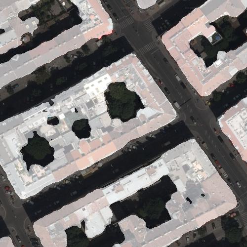
randomFile = RandomSample[FileNames["image/*.tif"], 1];
TestImage = Import[randomFile[[1]]];
TestMask = 
  Import[StringReplace[randomFile[[1]], "image/" -> "mask/"]];

Take 100 partition of the image to feed into the net:

imageToTest = ImagePartition[TestImage, {500, 500}];
maskToTest = ImagePartition[TestMask, {500, 500}];
rand1 = RandomInteger[{1, 10}];
rand2 = RandomInteger[{1, 10}];

ImageCompose[
 imageToTest[[rand1, 
  rand2]], {Image[netEvaluation[imageToTest[[rand1, rand2]]]], 0.5}]

ImageCompose[
 maskToTest[[rand1, 
  rand2]], {Image[netEvaluation[imageToTest[[rand1, rand2]]]], 0.5}]

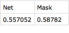
Compare the percentage of building in the area with the net and the mask:

{{"Net", "Mask"}, {ImageMeasurements[
    Image[netEvaluation[imageToTest[[rand1, rand2]]]], "Mean"], 
   ImageMeasurements[maskToTest[[rand1, rand2]], "Mean"]}} // Dataset

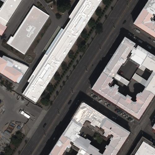
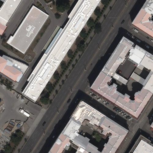
GeoImage

testImage[latitud_, longitud_, net_] := 
 Module[{geoImage, geoImageResize},
  geoImage = 
   GeoImage[GeoPosition[{latitud, longitud}], 
    GeoRange -> Quantity[75, "Meters"], GeoProjection -> "Mercator", 
    ImageSize -> Small];
  geoImageResize = ImageResize[geoImage, {500, 500}];
  {ImageCompose[geoImageResize, {Image[net[geoImageResize]], 0.3}]
   , Image[net[geoImageResize]]}]

IER-UNAM

IER = testImage[18.839940, -99.235635, netEvaluation]