Background
Automated reading of text, functions or even interpreting images has seen impressive improvements in the last years. For charts of various kinds, this has been much more difficult due to the multiple elements like lines that are overlapping, a neverending range of design choices and other problems making this a complicated task. This has various implications both for automated reading of printed media for various purposes, including applications for visually impaired individuals.
Approach
This kind of problem is incredibly complicated to tackle with traditional algorithms due to the complexity of styles, contrast, size of charts and much more, so I decided to try and solve this problem using machine learning. I ran into many problems at first, mostly because it took me several rounds of dataset generation until I figured out which parameters I needed to change to make the graph accurate for bar charts that were not generated by the Wolfram Language. Things like varying the amount of space above the highest bar, so the network didn't cheat on reading the number of the side. Or generating different image sizes, so the ratio of text to graph would change. The network is still not doing very well in detecting the specific numbers displayed in a bar chart if they are outside the range I used for my generated data, but it is an interesting proof of concept, that I hope I can build on in the future. Either with more and better training data, preprocessing of the images or a combination of the two.
The code
Dataset generation
The following code was used to export a large number of bar charts as jpg files, as well as mx-files containing the data they were generated with as solutions.
Image Size, Color, the distance between the top of the plot and the highest bar and a few other parameters are all chosen randomly.
Problems: the values are only between 100 and 1000. Different ranges could be generated to train the network to do more, but there are problems with smaller numbers becoming less significant in the loss function.
SeedRandom[123456];
randomList:=Table[{RandomInteger[{100,1000}],RandomWord[]},RandomInteger[{1,15}]];

dataset= ParallelTable[With[{j=CreateUUID[],rl=randomList},
    (Export[StringTemplate["C:\\Users\\rbc15\\Desktop\\Mathematica\\MLData3\\``.jpg"][j],
    Rasterize[BarChart[
    RandomChoice[{
rl[[All,1]],
Map[Labeled[#[[1]],#[[2]]]&,rl],
Map[Placed[Labeled[#[[1]],#[[1]]],Top]&,rl]
}],
    ChartStyle->RandomChoice[ColorData["Charting"]],
    ChartStyle->Thickness[RandomReal],
    Background->RandomChoice[{.8,.2}->{None,RandomColor[]}],
    ChartElementFunction->RandomChoice[ChartElementData["BarChart"]],
    BarSpacing->RandomChoice[{None,Automatic,Tiny,Small,Medium,Large}],
    PlotLabel->RandomChoice[WordList[]],
    PlotRange->Max[rl[[All,1]]]+RandomInteger[{0,4000}]
    ],ImageSize->RandomInteger[{100,400}]]];
       Export[StringTemplate["C:\\Users\\rbc15\\Desktop\\Mathematica\\MLData3\\``.mx"][j],
       rl[[All,1]]])],100000];
Turning files into a dataset
(*location of the data files*)
dataDirectory="C:\\Users\\rbc15\\Desktop\\Mathematica\\MLData3\\";
(*names of all the different plots I generated*)
ids=Map[FileBaseName,Map[FileNameTake,FileNames[___~~".mx",dataDirectory]]];
(*exporting a mx file with all the names of the data files*)
Export["C:\\Users\\rbc15\\Desktop\\Mathematica\\MLNamesData3.mx",ids]
(*creating an mx file with the data that generated the jpg files used for training,
 associated with their name*)
mxs=AssociationMap[Import[FileNameJoin[{dataDirectory,StringJoin[#,".mx"]}]]&,ids];
(*exporting those files as well*)
Export["C:\\Users\\rbc15\\Desktop\\Mathematica\\MLData3.mx",mxs]
Modifying nets to meet my needs
Now that I have some data to train my net with, I need a net to train. I looked through the repository and documentation to find nets that would meet my needs. I needed the final chart reader to output a list of numbers, but having a classifier seemed impossible, due to the almost inexhaustible number of possible outputs.
Instead, I split the problem into two sections, one ocr net that would read the relative height of the bars (for now in 20 different categories as fractions of the highest bar, but with the possibility of increasing this resolution.
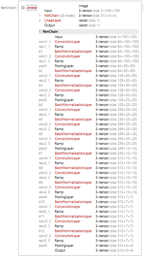
To scale the relative heights for the total height of the data, I used a modified image identification net (vgg-16 net trained on image competition data), cut off and added a few layers to make it return a single number representing the highest bar.
Below you can see the code creating the specific training sets and NetChains for the two networks and training them.
Defining the data, training set and test set for the first net
(*complete dataset*)
data=Flatten[Map[
    {File[FileNameJoin[{dataDirectory,StringJoin[#,".jpg"]}]]
    ->{Max[mxs[[Key[#]]]]}}&,ids]];
(*separate training and testing set *)
{training,testing}=TakeDrop[RandomSample[data],98000];
Doing the same for the second net
(*defining a function that takes a list of values and turns them into relative heights
to a given number of bins*)
class[list_,nbins_]:=Map[Floor[(#/Max[list])*nbins]&,list]
(*using the class function and my ids to associate each file with the list of its relative heights*)
listData=Flatten[Map[
    {File[FileNameJoin[{dataDirectory,StringJoin[#,".jpg"]}]]->class[mxs[[Key[#]]],20]}&,
         ids]];
(*splitting the dataset in the same number of training and testing data as before*)
{traininglist,testinglist}=TakeDrop[RandomSample[listData],98000];
Modifying the vgg-16 net
(*Importing vgg16Net as a base for my network*)
vgg16Net= NetModel["VGG-16 Trained on ImageNet Competition Data","UninitializedEvaluationNet"]
(*cutting off a few layers at the end to match the output form I want (one number)*)
vgg16Net2= NetReplacePart[NetTake[vgg16Net,{"conv1_1","pool5"}],
"Input"->NetEncoder[{"Image",100}]];
(*Adding a BatchNormalizationLayer before every ConvolutionLayer*)
vgg16Net3=NetInsert[vgg16Net2,"b1"->BatchNormalizationLayer[],"conv1_2"];
vgg16Net3=NetInsert[vgg16Net3,"b2"->BatchNormalizationLayer[],"conv2_1"];
vgg16Net3=NetInsert[vgg16Net3,"b3"->BatchNormalizationLayer[],"conv2_2"];
vgg16Net3=NetInsert[vgg16Net3,"b4"->BatchNormalizationLayer[],"conv3_1"];
vgg16Net3=NetInsert[vgg16Net3,"b5"->BatchNormalizationLayer[],"conv3_2"];
vgg16Net3=NetInsert[vgg16Net3,"b6"->BatchNormalizationLayer[],"conv3_3"];
vgg16Net3=NetInsert[vgg16Net3,"b7"->BatchNormalizationLayer[],"conv4_1"];
vgg16Net3=NetInsert[vgg16Net3,"b8"->BatchNormalizationLayer[],"conv4_2"];
vgg16Net3=NetInsert[vgg16Net3,"b9"->BatchNormalizationLayer[],"conv4_3"];
vgg16Net3=NetInsert[vgg16Net3,"b10"->BatchNormalizationLayer[],"conv5_1"];
vgg16Net3=NetInsert[vgg16Net3,"b11"->BatchNormalizationLayer[],"conv5_2"];
vgg16Net3=NetInsert[vgg16Net3,"b12"->BatchNormalizationLayer[],"conv5_3"];
(*Adding a LinearLayer[1] as the last layer*)
vgg16Net4=NetChain[{vgg16Net3,LinearLayer[1]}]
Let's train it!
vgg16NetTrained=NetTrain[vgg16Net4,training,ValidationSet->testing,
                 TargetDevice->"GPU",BatchSize->32]
Export["MaxLength4.wlnet",vgg16NetTrained]
To see if it successfully reads the highest point in the graphs, even though those change relative to the axis, I made a table with the input, output, expected output and percentage error.
sample=RandomSample[testing,10];
Grid[Prepend[Map[{Show[Import[#[[1]]],ImageSize->200],vgg16NetTrained[#[[1]]],#[[2]],
       ((vgg16NetTrained[#[[1]]]-#[[2]])/#[[2]]*100)}&,sample],
{"Input", "Output", "expected Output","Percentage Error"}],Frame->All]
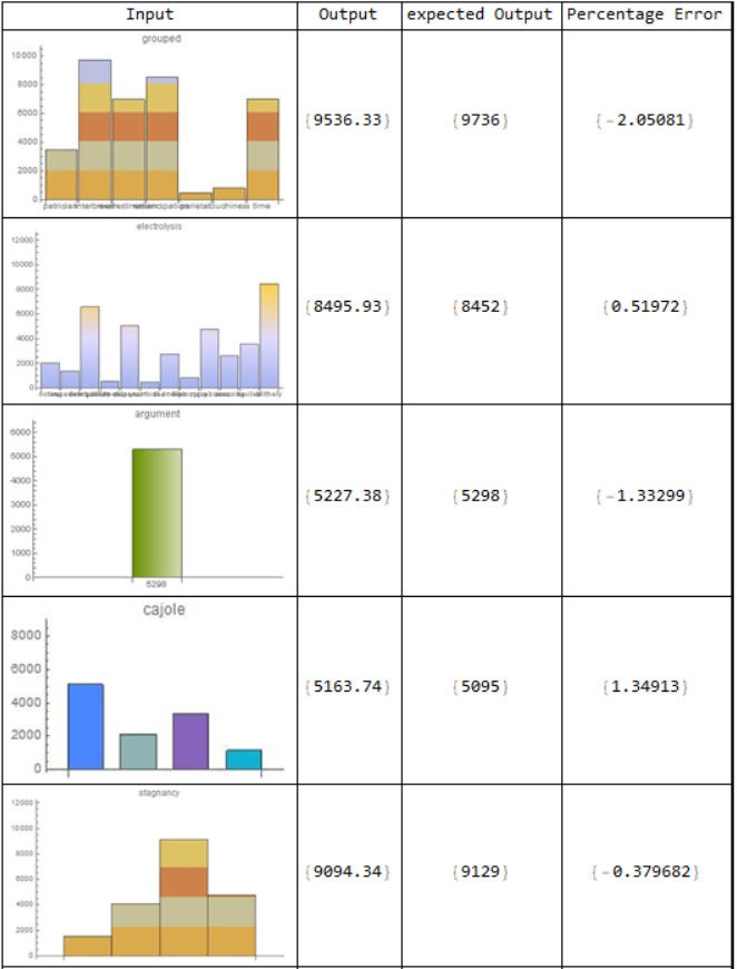
It worked reasonably well, for the range I gave it, but is of course specialized to these numbers now, as I will show later.
Let's do the same for the second net!
generating and training an ocr net
(*defining a few building blocks for the network*)
loss=CTCLossLayer[];
classes=Range[20];
decoder=NetDecoder[{"CTCBeamSearch",classes}];
convUnit[c_]:=NetChain[{ConvolutionLayer[c,3],BatchNormalizationLayer[],Ramp,PoolingLayer[2]}]
(*putting the net together*)
ocrNet=NetChain[{convUnit[50],convUnit[50],convUnit[50],convUnit[50],convUnit[10],
    TransposeLayer[1<->3],FlattenLayer[-1],GatedRecurrentLayer[50],GatedRecurrentLayer[50],
    NetMapOperator[LinearLayer[Length[classes]+1]],SoftmaxLayer[]},
    "Input"->NetEncoder[{"Image",100,"Grayscale"}],"Output"->decoder]
(*training the net*)
ocrNetTrained=NetTrain[ocrNet,traininglist,ValidationSet->testinglist,LossFunction->loss,BatchSize->32,TargetDevice->"GPU"]
Export["RelativeHeight4.wlnet",ocrNetTrained];
Testing it
(*defining a sample of the list data*)
samplelist=RandomSample[testinglist,10];
(*visually representing the output of the network reading the relative heights*)
Grid[Prepend[Map[
    {Show[Import[#[[1]]],ImageSize->200],BarChart[ocrNetTrained[#[[1]]]],BarChart[#[[2]]]}&,samplelist],
    {"Input", "Output", "expected Output"}],Frame->All]
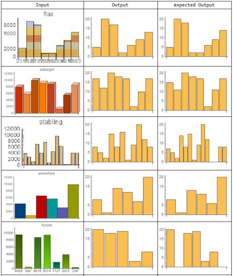
This net also does a reasonably good job, but the given examples already illustrate a few problems it is encountering. For example not being able to distinguish between one or two bars of the same height in the first bar chart or cutting out very low bars in the third or fifth example.
One reason for this is likely that it does not even have a category for a relative height of zero (less than a 20th of the highest bar) as well as such low bars not being very significant for the loss function.
Even if there is still lots to improve, I put the two networks together in a function that can read pictures of bar charts and turn them into new bar charts.
First, I tried this on the sample from my testing set:
readGraph[graph_]:=Flatten[Map[#*(vgg16NetTrained[graph]/20)&,ocrNetTrained[graph]]]
SetAttributes[readGraph,Listable]
Grid[Prepend[Map[{Show[Import[#],ImageSize->200],BarChart[readGraph[#]]}&,sample[[All,1]]],
    {"Input", "Output"}],Frame->All]
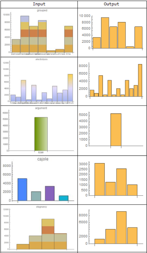
This also seems to be working reasonably well, even though the flaws of both networks are combining and making it even more fault-prone.
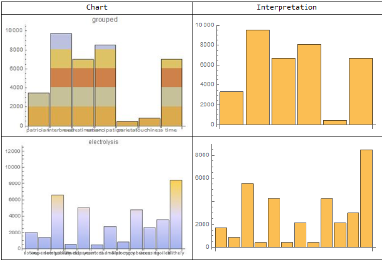
To see how this function would perform on graphs not generated using the Wolfram Language, I used WebImageSearch to test it on a few examples from the web.
Grid[Prepend[Map[{Show[#,ImageSize->200],BarChart[readGraph[#]]}&,
WebImageSearch["Bar Chart", "Thumbnails",MaxItems->10]],{"Chart","Interpretation"}],
    Frame->All]
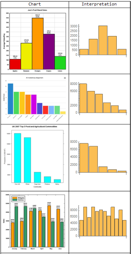
It is doing something with the images. Many of the same problems exist, like the inability to read graphs of the same height, as well as some new problems, like the new scale of the images and different kinds of noise , such as writing, different chart width, and many more.
Conclusion
There are many problems to be solved in the approach I am taking, but the project shows the possibilities Machine Learning opens in this complex task. I hope to train and develop this net further to get lower error rates and read a further array of graphs.
Thank you for reading the community post.
The code can also be found on my github
 Attachments:


