Introduction
The goal of this project was to come up with an algorithm to describe time series data in natural language. Humans can look at a plot of data and come up with a general description of what it's doing with very little effort. This is much harder for computers; specifically the idea of a "general" description is something that is not well defined. How exactly do you get a general description from specific data points?
Principles
This is an extremely open-ended problem, and could be tackled in a number of ways. Here I will describe some of the design principles that informed my approach:
Local vs. Global Features:
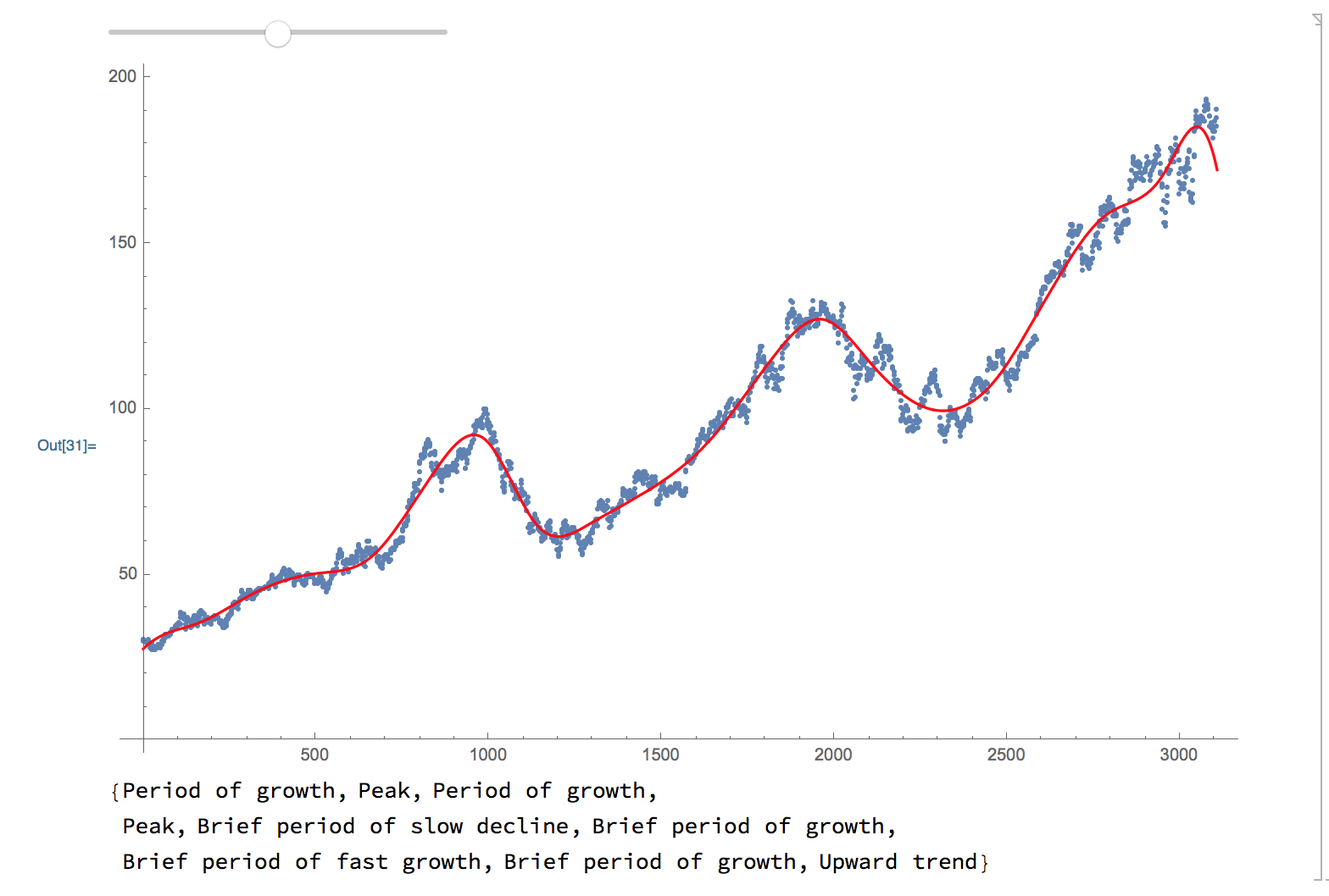
If a person were to describe the data pictured above, Apple stock from 2010 until now, they would likely say that there is a general upward trend, with a few significant peaks. I wanted my algorithm to be able to distinguish local and global features.
Robust to Noise
The standard way that the computer represents this data is to hold the exact value of every point. As such every fluctuation is recorded, no matter how small. However, describing the graph in this way would be extremely tedious. I wanted my algorithm to be able to think of very close points as being essentially the same; in other words it should be robust to noise.
Arbitrary Detail
Humans can easily give a more or less detailed description of the same data, and have little trouble deciding what details can and cannot be ignored. I wanted my algorithm to be similarly capable of changing the level of detail in the description.
Overview
Here is a brief overview of what my algorithm does:
- Fit the data to a sum of a linear function and piecewise polynomials.
- Classify the local features in a "fuzzy" way.
- Split these features into sections.
- Generate descriptive words for these sections.
Piecewise Fit
The algorithm first subtracts from the data the linear least squares fit, to measure global trends. It then fits this "de-trended" data with a weighted sum of cubic b-spline basis functions, evenly spaced along the x-axis, which have local support and can thus model local features well. The number of b-spline basis functions used can be tweaked by the user to get a more or less detailed description. Mathematically this fit can be described as follows:
$$ a x+b+\sum _i^n c_i N_3\left(x-t_i\right) $$
Where $a$ and $b$ are coefficients of the linear least squares fit, $N_3(x)$ is the cubic b-spline basis function, $t_i$ is the center of the $i$th basis function, and $n$ is the user-controlled number of b-spline basis functions to fit.
Below is the code used to generate this fit:
base[center_, support_, x_] := N[BSplineBasis[3, (1./support)*(x-center) + 1/2]]

piecewiseCoeffsWLinear[nPts_, data_]:=
    Block[{dom, length, basisMat, linFit, fixedData},

       (*calculate linear fit*)
       linFit = LinearModelFit[data, xp, xp];

       (*subtract linear fit from data*)
       fixedData = {#1, #2 - linFit[#1]}&@@@data;

       (*fit leftovers with sum of splines*)
       dom = data[[-1,1]] - data[[1,1]];
       length = Length@data;
       basisMat = SparseArray[Table[base[dom*(c-1)/(nPts-1)+data[[1,1]], 4 dom/nPts, data[[r, 1]]], {r, length}, {c, nPts}]];
       {LeastSquares[basisMat, fixedData[[All, 2]]], Abs[linFit["BestFitParameters"][[2]]*dom]}
    ]
Fuzzy Classification
Once the coefficients of these functions are obtained, they are classified into one of seven bins, "big positive", "medium positive", "small positive", "near zero", ... , "big negative". This classification is done in the style of fuzzy set theory, where each bin has a "membership function", which assigns to each coefficient a number from 0 to 1, indicating how much the coefficient belongs in that set. The boundaries of these functions overlap, so one coefficient might belong to "medium positive" with a value of 1, but also to "big positive" with a value less than 1. This sort of "fuzzy classification" mirrors how humans describe similar situations; there is no cutoff value where a number stops being small and becomes big. Practically, this allows the system to be robust to noise, as any noise will not affect classification much. It also allows for context-dependent segmentation of the data; if one coefficient is "medium positive" with value 1, and "big positive" with value less than one, if it is near other "big positive" values it may be interpreted similarly.
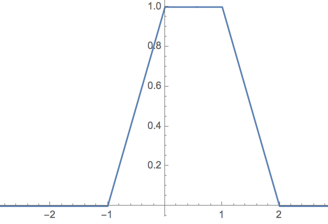
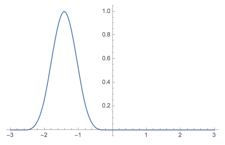
Here is code representing the membership function of some bin:
membership[x_, width_] := Ramp[x/width + 1] - UnitStep[x]Ramp[x/width] - UnitStep[x-width]Ramp[x/width - 1] + UnitStep[x-2width]Ramp[x/width - 2]
And here is a function to classify some $x$ into some $n$ evenly spaced bins:
classify[x_, n_, min_, max_]:=
With[{range = max - min},
    membership[x - (#-1.)/(n) range - min, range/(n)]&/@Range[n]
]
Segmentation
The next step is to calculate a "fuzzy derivative" over these classifications. This is essentially a weighted sum, which returns sort of an "average value" of how much the function increased from one point to another. This is where the context-dependence kicks in. Once this is calculated, the program segments the data into stretches based on sudden changes in this fuzzy derivative. Each of these segments represents a stretch of roughly constant activity, whether that's a flat section, a sharp increase or decrease, etc.
The "fuzzy derivative" is computed as follows:
delta[x_, y_] :=
With [{len = Length@x},
    Map[Max,
       Map[x[[#]]&, Table[i, {i, Max[1, 1-#], Min[len, len-#]}]&/@(Range[2len-1]-len)]*
       Map[y[[#]]&, Table[i + #, {i, Max[1, 1-#], Min[len, len-#]}]&/@(Range[2len-1]-len)]
    ]
]
These segments are then classified (definitively) as either "sharply increasing", "increasing", "flat", "decreasing", or "sharply decreasing". This is represented by an integer from -2 to 2. The number of splines belonging to that segment is also recorded as the relative length of that segment. Additionally, the program records the ratio of increase in the linear fit model, to the largest local fluctuation. This ratio ranks the importance of local to global structure in the data.
Text Description
This is the "semantic information" that the algorithm extracts from the data, and represents numerically how a human might describe the data. The next step would then be to turn that information into words. I didn't put as much time and energy into this part of the project, but some simple pattern matching can be used to change sequences of "up, down, up, down, ..." into "oscillations", "peaks", and "valleys". The rest of the info is then replaced with phrases such as "brief period of fast growth", "period of slow decline", etc. Certainly it wouldn't be very difficult to take this information and stitch it into a better, more natural sounding sentence.
Here is code for this simple word replacement scheme:
wordify[semantics_]:=
    Block[{firstpass},
       firstPass = SequenceReplace[semantics[[1]], {Repeated[{{_, {2}}, {_, {-2}}}, {2, Infinity}]-> "large oscillation",
                              Repeated[{{_, {-2}}, {_, {2}}}, {2, Infinity}]-> "large oscillation",
                              Repeated[{{_, {1}}, {_, {-1}}}, {2, Infinity}]-> "small oscillation",
                              Repeated[{{_, {-1}}, {_, {1}}}, {2, Infinity}]-> "small oscillation",
                              {{_, {2}}, RepeatedNull[{1|2, {-1|0|1}}, 1], {_, {-2}}}-> "peak",
                              {{_, {-2}}, RepeatedNull[{1|2, {-1|0|1}}, 1],
                              {_, {2}}} -> "valley"}];

       secondPass = {Replace[Replace[firstPass, heightWords, {2}], lengthWords, All], semantics[[2]]}
    ]
All of this functionality is wrapped up neatly in the (quite long) function:
dataToWords[data_, detail_]:=
    Block[{info, lengthWords, coeffs, secondPass, firstPass},
       coeffs = piecewiseCoeffsWLinear[detail, data];
       info = Map[classify[#, 7, Min@coeffs[[1]], Max@coeffs[[1]]]&, coeffs[[1]]];
       info = Map[(Range[13]-7).#&, Map[delta[info[[#]], info[[#+1]]]&, Range[Length@info-1]]];
       info = Map[Round, Map[{Length[#], Mean[#]}&, Split[info, (Abs[#1- #2] <=  2.1)&]]];
       info = Apply[{#1, classify[#2, 5, Min[info[[All,2]]], Max[info[[All,2]]]]}&, info, {1}];
       info = Apply[{#1, Position[#2,Max@#2][[1]]-3}&, info, {1}];
       lengthWords = lengthWordsTemplate[detail];
       firstPass = SequenceReplace[info, {Repeated[{{_, {2}}, {_, {-2}}}, {2, Infinity}]-> "Large oscillation",
                              Repeated[{{_, {-2}}, {_, {2}}}, {2, Infinity}]-> "Large oscillation",
                              Repeated[{{_, {1}}, {_, {-1}}}, {2, Infinity}]-> "Small oscillation",
                              Repeated[{{_, {-1}}, {_, {1}}}, {2, Infinity}]-> "Small oscillation",
                              {{_, {2}}, RepeatedNull[{1|2, {-1|0|1}}, 1], {_, {-2}}}-> "Peak",
                              {{_, {-2}}, RepeatedNull[{1|2, {-1|0|1}}, 1],
                              {_, {2}}} -> "Valley"}];
       secondPass = Replace[Replace[firstPass, heightWords, {2}], lengthWords, All];
       Join[Quiet[secondPass /. {a_String,b_String}->a<> " of "<>b], {ratioDesc[coeffs[[2]]/Max[Abs[coeffs[[1]]]]]}]
    ]
Conclusion
The semantic information obtained from this method is robust to noise, and is a good indicator of how a human might describe a plot of the data. It distinguishes local and global features, and can be made into a proper sounding sentence with a sequence of replacement rules and grammatical operations. This scheme is also fast, analyzing sets of 2000 data points in around 500 ms. The system for going from semantic information to words is very simplistic, and could be greatly improved. Additionally, a system for iteratively more detailed fitting could allow for a more detailed description without over-fitting. Finally, mapping this description to the original domain of the data would be very useful, so that a description like "there was a peak around 2009" would be possible.
 Attachments:


