Introduction
We attempted to generate a certain type of boundary conditions, such as those in partial differential equations, to apply cellular automata (CA) rules in regions contained by arbitrary boundaries. These boundaries could be irregular, and may interact with the units inside. Two cellular automata were constructed and studied in particular, a simple forest fire model as a probabilistic CA and fluid flow as an hexagonal CA. Code from existing demonstrations was modified to apply them to arbitrary regions.
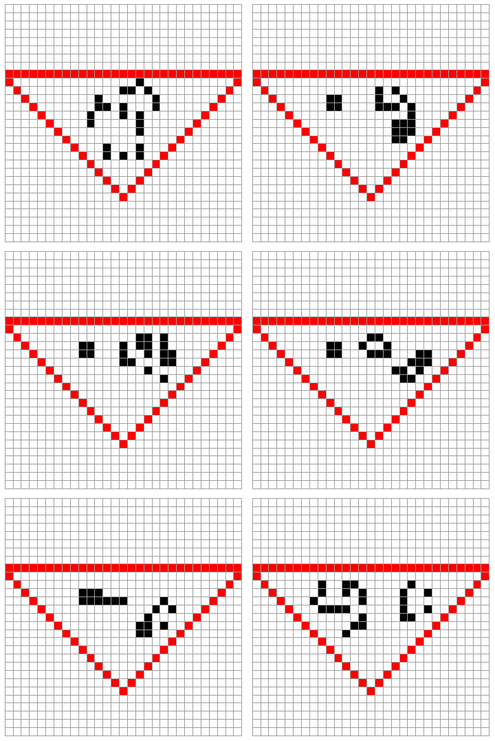
We focused in 2D cellular automata. Similar to the two cases mentioned above, Conway's Game of Life CA was implemented to arbitrary regions defined by an image or different values on an array. The code below shows the set of rules needed to run Game of Life inside a triangle.
ruleTriangleBoundary[matrix_] :=
 Module[{m = matrix, neighbours,
   a = Floor[Dimensions[matrix][[1]]/3]},
  neighbours =
   ListConvolve[{{1, 1, 1}, {1, 0, 1}, {1, 1, 1}}, ArrayPad[m, 1]];
  m = ReplacePart[m,
    Position[neighbours, _?(# < 2 || # > 3 &)] -> 0];
  m = ReplacePart[m, Position[neighbours, 3] -> 1];
  m = ReplacePart[m, {a, i_} -> -1];
  m = ReplacePart[m,
    Thread[Table[{i + a, i}, {i, 1, Length@m/2}] -> -1]];
  m = ReplacePart[m,
    Thread[Table[{i + a + 1, Length[m] - i}, {i, 0,
        Length@m/2}] -> -1]]
  ]
One can display the set of rules by giving an initial state as a 2D array of values.
m = ArrayPad[RandomInteger[1, {9, 9}], 10];
ltriangle =
  ArrayPlot[#, Mesh -> True,
     ColorRules -> {1 -> Black, 0 -> White, -1 -> Red}] & /@
   NestList[ruleTriangleBoundary, m, 100];
Manipulate[ltriangle[[n]], {n, 1, 50, 1}, ImageMargins -> 32,
 FrameMargins -> 30, ContentSize -> Large]

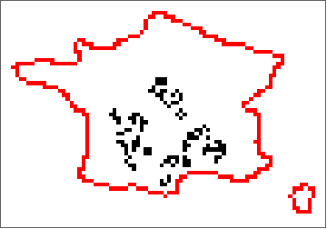
What if we want to give this an arbitrary boundary region. We could take a region from an image and set up the set of rules for the boundaries desired. Say for instance one wants to implement a simple set of rules so that Conway's Game of Life cellular automata is contained to a certain arbitrary region in 2D. Below different regions are transformed as positions of an array or matrix where the cellular automata interacts.
(*Image import*)
image = Graphics[Interpreter["Country"]["France"]["Polygon"]];
newimage = ColorNegate@EdgeDetect[ImageResize[image, {80}]]
matrix = ImageData[newimage];
matrix = Replace[matrix, {0 -> 1, 1 -> 0}, Infinity];

(*Boundary rules generated*)
boundary[matrix_] := Thread[Position[matrix, 1] -> -1];
boundaryrules = boundary[matrix];
dim = Dimensions[matrix];

(*updating function based on rules*)
randomImage[matrix_] :=
 Module[{m = matrix, neighbours},
  neighbours =
   ListConvolve[{{1, 1, 1}, {1, 0, 1}, {1, 1, 1}}, ArrayPad[m, 1]];
  m = ReplacePart[m,
    Position[neighbours, _?(# < 2 || # > 3 &)] -> 0];
  m = ReplacePart[m, Position[neighbours, 3] -> 1];
  m = ReplacePart[m, boundaryrules]
  ]
For this then one needs to make sure the dimensions of the initial state matrix and the one from the image have to have same dimensions.
(*Initial state matrix*)
minitial = PadLeft[
   Table[RandomInteger[
     1], {Floor[dim[[1]]/3]}, {Floor[dim[[2]]/3]}], {dim[[1]],
    dim[[2]]}, 0, {Floor[dim[[1]]/3], Floor[dim[[2]]/3]}];

limage = ArrayPlot[#,ColorRules -> {1 -> Black, 0 -> White, -1 -> Red}, ImageSize -> Medium] & /@
NestList[rulesrandomImage, minutial, 50];
ListAnimate[limage]
This simple code is just a proof of concept, by adding an extra set of rules and/or values to the boundary units one can apply known cellular automata in arbitrary units.

Now looking at the modified demonstrations, additional states and rules gave interesting cellular automata in arbitrary regions.
Forest Fire
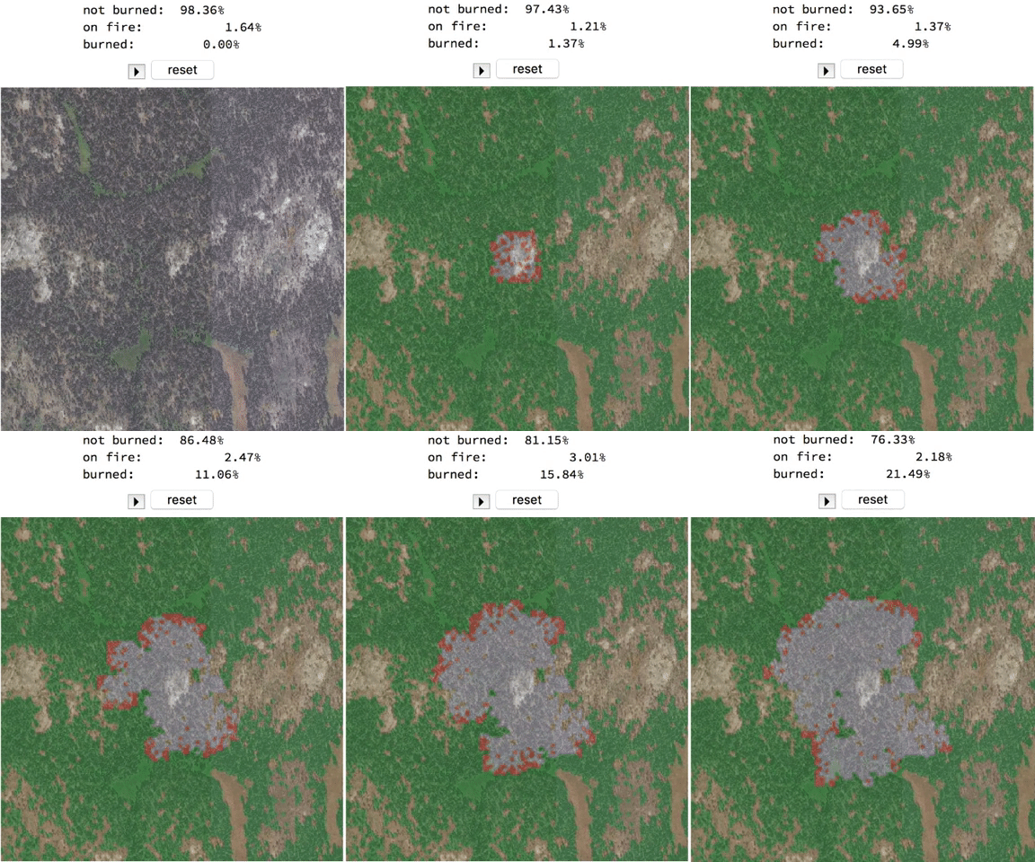
A probabilistic forest fire cellular automata was modified to allow one extra state to define regions were the tree units could burn. Previously it allowed for 3 possible states: unburnt tree, burnt tree, and burning tree, where the probability of the last two was given by the "ignite" and "staylit" parameters, respectively. One extra state was added and to maintain a constant region that could not be affected by the "active" neighbor units/trees. This region was determined from an actual map or satellite image from a forest.
With this code a digital satellite image of the Giant Forest in California is imported.
image2 = GeoImage[Interpreter["Forest"]["Giant Forest"],
   GeoRange -> Quantity[0.5, "Miles"], GeoServer -> "DigitalGlobe",
   ImageSize -> Medium ];
image = Binarize@ImageResize[image2, {100, 100}]
imagedata = ImageData[image2new] /. {1 -> 3};
The image is binarized and the area that is not green is turned into a state that cannot burn. The manipulate code takes the image and overlays a simulation of a set of burning trees in the center. This can be seen in the gif below.
Manipulate[
 Module[{iteration}, SeedRandom[1]; SetAttributes[setPart, HoldFirst];
   setPart[sym_, {x_, y_}, value_] := sym[[x, y]] = value;
  iteration :=
   Module[{}, ((trees[[Sequence @@ #1]] =
          RandomChoice[{staylit, 1 - staylit} -> {1, 2}];) &) /@
     Position[trees,
      1]; ((Do[
          Which[MemberQ[#1 + i, 0 | 101], Null,
           trees[[Sequence @@ (#1 + i)]] == 3, Null,
           trees[[Sequence @@ (#1 + i)]] == 0,
           setPart[trees, #1 + i,
            RandomChoice[{1 - ignite, ignite} -> {0, 1}]]], {i,
           DeleteCases[Tuples[{-1, 0, 1}, 2], {0, 0}]}];) &) /@
     Position[trees, 1]];
  Column[{Dynamic[
     Column[{Row[{"not burned: ",
         NumberForm[
          Round[N[100/(10000 - Count[Flatten[trees], 3])
              Count[Flatten[trees], 0]], .01], {4, 2},
          NumberPadding -> {" ", "0"}], "%"}],
       Row[{"on fire:         ",
         NumberForm[
          Round[N[100/(10000 - Count[Flatten[trees], 3])
              Count[Flatten[trees], 1]], .01], {4, 2},
          NumberPadding -> {" ", "0"}], "%"}],
       Row[{"burned:       ",
         NumberForm[

          Round[N[100/(10000 - Count[Flatten[trees], 3])
              Count[Flatten[trees], 2]], .01], {4, 2},
          NumberPadding -> {" ", "0"}], "%"}]}]],
    Row[{Animator[
       Dynamic[run, (iteration; run = #1) &], {0, \[Infinity], 1},
       AppearanceElements -> {"PlayPauseButton"},
       DisplayAllSteps -> True, AnimationRepetitions -> 1,
       DefaultDuration -> 2, PausedTime -> 0],
      Button["reset", trees = imagedata;
       trees[[45 ;; 55, 45 ;; 55]] = 1;]}],
    Dynamic[ImageCompose[
      image2, {ImageResize[
        Graphics[
         Raster[Reverse[
           Developer`ToPackedArray[
            trees /. {0 -> {0., .6, 0.}, 1 -> {1., .2, 0.},
              2 -> {.8, .8, .8}, 3 -> {.5, .4, .1}}]]],
         PlotLabel -> None, PlotRange -> {{0, 100}, {0, 100}},
         ImageSize -> 600
         ], ImageDimensions[image2]], 0.3}], {600, 600}]},
   Center]], {{ignite, .7, "chance to catch on fire"}, .1, .9,
  Appearance -> "Labeled"}, {{staylit, .45,
   "chance to stay on fire"}, .1, .9,
  Appearance -> "Labeled"}, {{trees,
   ReplacePart[imagedata,
    Partition[Flatten[Table[{i, j}, {i, 45, 55}, {j, 45, 55}]], 2] ->
     1]}, ControlType -> None}, {run, 0, 10, 1, ControlType -> None},
 TrackedSymbols -> Manipulate, AutorunSequencing -> {4},
 ContentSize -> Large]

Fluid Flow Cellular Automaton
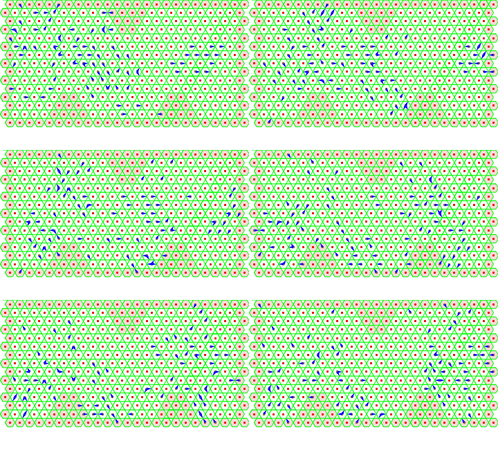
A fluid flow manipulate model was modified to allow the user to choose from four different configurations. This model in an hexagonal grid is similar as that discussed by Stephen Wolfram in NKS. The interaction rules of the particles take partially into consideration the conservation of momentum and energy. A set of reflections rules were defined to the interaction of particles with walls defined by 3 configurations. The manipulate lets the user control the steps of the model as well as the Random Seed that sets up the initial state of the simulation. Since the initialization and manipulate code is a little bit long this was attached as files that you can download.
Conclusion
The boundary conditions for all implementations where done by adding extra rules of interaction between units in a grid or directly as a cellular automata structure. These additional rules interacted in different ways with the other units. Analogies to the way Boundary Conditions are defined for Partial Differential Equations could be made. For instance, fixing the values of the boundary units can be though of fixing the values of a function in a certain region. Similarly defining the rules that determine the change in the values of the units can be though of as defining the derivative of a function in a region or boundary. Moreover, for the Forest Fire simulation and extra state was added but this would be set to remain constant. No interaction rules were given to these boundary units or units within the regions that could not burn in the model. This could be defined as a Dirichlet Boundary Condition since the values of the "function" are defined in a region.
Future Work
Some studies of these type of boundary conditions have been done for Boolean CA, however studying in more detail these kind of boundary conditions can result in more interesting cellular automata. Just like for Partial Differential Equations, one could classify these types of boundary conditions for CA. Other types of boundary conditions could be constructed and studied. For instance, one could construct a 2D cellular automata in the surface of a sphere or torus, by setting certain transformations and periodic boundary conditions.
Data and Code Sources Links/References
https://arxiv.org/pdf/1606.05122.pdf http://www.stephenwolfram.com/publications/academic/cellular-automaton-fluids-theory.pdf http://demonstrations.wolfram.com/CellularAutomatonFluids/ http://demonstrations.wolfram.com/AProbabilisticForestFireModel/
 Attachments: