Author: Nikhil Gaddam
Introduction
Greetings all,
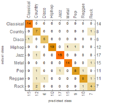
This year at the Wolfram Summer Camp I studied audio classification using machine learning in the wolfram language. My project focused on using a combination of a convolutional neural network and recurrent neural network to classify an audio clip into one of nine genres: classical, country, disco, hiphop, jazz, metal, pop, reggae, or rock. Since there had been little prior research into audio classification, the project presented many challenges however, I greatly enjoyed overcoming them. My finished neural network has an 85% accuracy when tested on a validation set of 100 songs.
You can test it out on your own music here: https://www.wolframcloud.com/objects/nikgad123/musicClassifier (Currently the website is not working due to wolfram cloud services issues)
Below is the confusion matrix plot of the neural net representing the genres it predicted compared to the actual genre of the test data.
Dataset
For my project I used the GTZAN dataset consisting of 1000 songs across 10 different genres (blues, classical, country, disco, hiphop, jazz, metal, pop, reggae, and rock) [1]. This is the most commonly used dataset in music classification projects,however the music in it is slightly outdated and not fully representative of modern music.
bluesFiles=FileNames["*.au",NotebookDirectory[]<>"genres\\blues"];
classicalFiles=FileNames["*.au",NotebookDirectory[]<>"genres\\classical"];
countryFiles=FileNames["*.au",NotebookDirectory[]<>"genres\\country"];
discoFiles=FileNames["*.au",NotebookDirectory[]<>"genres\\disco"];
hiphopFiles=FileNames["*.au",NotebookDirectory[]<>"genres\\hiphop"];
jazzFiles=FileNames["*.au",NotebookDirectory[]<>"genres\\jazz"];
metalFiles=FileNames["*.au",NotebookDirectory[]<>"genres\\metal"];
popFiles=FileNames["*.au",NotebookDirectory[]<>"genres\\pop"];
reggaeFiles=FileNames["*.au",NotebookDirectory[]<>"genres\\reggae"];
rockFiles=FileNames["*.au",NotebookDirectory[]<>"genres\\rock"];

blues=Import/@bluesFiles;
classical=Import/@classicalFiles;
country=Import/@countryFiles;
disco=Import/@discoFiles;
hiphop=Import/@hiphopFiles;
jazz=Import/@jazzFiles;
metal=Import/@metalFiles;
pop=Import/@popFiles;
reggae=Import/@reggaeFiles;
rock=Import/@rockFiles;

justAudio=Join[blues,classical,country,disco,hiphop,jazz,metal,pop,reggae,rock];

audioClasses={"Blues","Classical","Country","Disco","Hiphop","Jazz","Metal","Pop","Reggae","Rock"}
After getting the files I attributed each audio file to their respective genre, creating a list of associated files.
data=Join[
Thread[blues->"Blues"],
Thread[classical->"Classical"],
Thread[country-> "Country"],
Thread[disco-> "Disco"],
Thread[hiphop-> "Hiphop"],
Thread[jazz->"Jazz"],
Thread[metal->"Metal"],
Thread[pop->"Pop"],
Thread[reggae-> "Reggae"],
Thread[rock-> "Rock"]];
Audio Feature Extraction
Spectrogram
Spectrograms are visual graphs of audio often with time along the x axis and frequency of sound waves along the y axis. The intensity of each note is then represented by the intensity of color at each point on the graph. Here are some examples of my data: 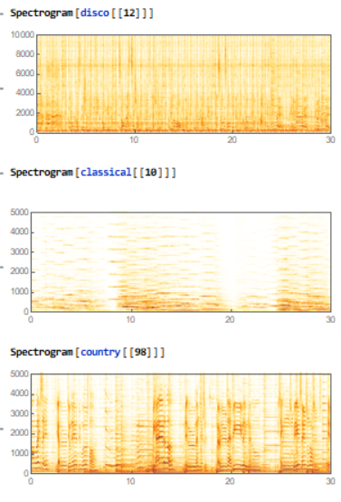
Mel Spectrogram
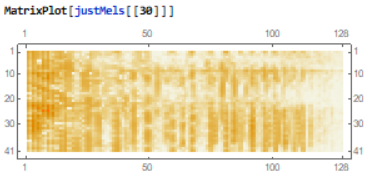
Audio Mel Spectrograms represent sound by applying a series a transformations on sound waves to achieve a power spectrum representation of the audio. It is said to better represent how humans interpret sound.
MFCC (Mel Frequency Cepstral Coefficients)
MFCC make up the coefficients or amplitudes of waves along the mel spectrum.
Building Neural Networks
Since genres are often classified by how a piece of music changes over time rather than a singular clip I decided to use a recurrent neural network. Recurrent Neural Networks (RNN) are especially good at identifying patterns in data and time dependent problems. They utilize Long Short Term Memory Layers (LSTMs) in their architecture to store data at different time intervals. I partitioned the audio files into 41 subsections to represent music at different time intervals.
RNN Network
First, I preprocessed the data before passing it into the net. This included attributing the blues audio files to "Jazz" music since blues is a sub type of jazz.
(* attributed blues to jazz music, since it is a specific type of jazz

 + previous methods were confusing the two classes often*)
data2=List[
Thread[blues->"Jazz"],
Thread[classical->"Classical"],
Thread[country-> "Country"],
Thread[disco-> "Disco"],
Thread[hiphop-> "Hiphop"],
Thread[jazz->"Jazz"],
Thread[metal->"Metal"],
Thread[pop->"Pop"],
Thread[reggae-> "Reggae"],
Thread[rock-> "Rock"]];

(* Take a random sample and convert all audio into MFCC*)
res2=RandomSample[data2];
justAudio2=#[[1]]&/@res2;
justClasses2=#[[2]]&/@res2;


enc2=NetEncoder[{"AudioMFCC",WindowSize->512,"NumberOfCoefficients"->20,"TargetLength"->41*68}]
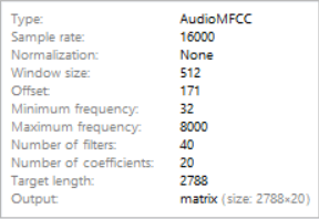
justMfcc2=enc2/@justAudio2;
justSplit2=Partition[#,41]&/@justMfcc2;

(*Reattribute partitioned data to classes*)
threaded2=Thread[justSplit2->justClasses2];
finalThreaded2=Thread/@threaded2;
finalData2=Flatten[finalThreaded2];
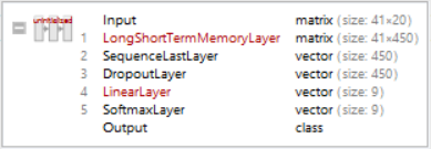
The architecture of this net is fairly simple. It uses a series of LSTMs, and retrieves the output of the last cell. It then uses a dropout layer to turn off certain weights and biases in the neural net to prevent overfitting. This is then sent to a Linear Layer with 9 nodes, each representing the different genres and finally to a SoftMax Layer which converts the results into understandable probabilities.
rnnNet4=NetChain[{
LongShortTermMemoryLayer[450],

SequenceLastLayer[],

DropoutLayer[0.5],


LinearLayer[9],
SoftmaxLayer[]
},
"Input"->{41,20},
"Output"->NetDecoder[{"Class",newclasses}]
]
trainData2=finalData2[[;;50000]];
testData2=finalData2[[50000;;51000]];

(*fully trained network*)
rnnTrained4=NetTrain[rnnNet4,trainData2,ValidationSet->testData2,TargetDevice->"GPU",MaxTrainingRounds->30]
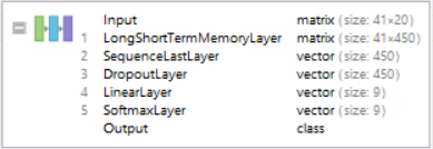
The neural net had an accuracy of 65% on the validation set.
Final Neural Network
I chose a new architecture based on a neural net which had been used fairly successfully on instrument recognition [2]. This combined both a convolutional neural network (CNN) and recurrent neural network (RNN).
First. I trained a CNN which took in a partitioned mel spectrograms and did its "learning" through a series on hidden and pooling layers. A CNN is especially useful in minimizing the amount of data in a neural network while still extracting key information. For example, it might use a kernel to reduce the dimensions of a tensor while still accounting for weights and biases. I chopped off the last output layer of this network which converted the many matrices into classes and probabilities.
CNN Training
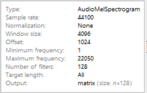
(* used a higher sampling rate and window size for this encoder to improve quality of data extraction*)

enc2=NetEncoder[{"AudioMelSpectrogram","WindowSize"->4096,"Offset"->1024,"SampleRate"->44100,"MinimumFrequency"->1,"MaximumFrequency"->22050,"NumberOfFilters"->128}]
justMels2=enc2/@justAudio2;
justSplit2=Partition[#,41]&/@justMels2;
threaded2=Thread[justSplit2->justClasses2];
CNN Architecture
conv[n_]:=NetChain[{ConvolutionLayer[n,{3,3},"Stride"->1,"PaddingSize"->2],Ramp}]

cnnNet=NetChain[
{
conv[32],
conv[32],
PoolingLayer[{3,3},"Stride"->3,"Function"->Max],
BatchNormalizationLayer[],
Ramp,
conv[64],
conv[64],
PoolingLayer[{3,3},"Stride"->3,"Function"->Max],
BatchNormalizationLayer[],
Ramp,
conv[128],
conv[128],
PoolingLayer[{3,3},"Stride"->3,"Function"->Max],
BatchNormalizationLayer[],
Ramp,
conv[256],
conv[256],
PoolingLayer[{3,3},"Stride"->3,"Function"->Max],
BatchNormalizationLayer[],
Ramp,
LinearLayer[1024],
Ramp,
DropoutLayer[0.5],
LinearLayer[9],
SoftmaxLayer[]
},
"Input"->{1,41,128},
"Output"->NetDecoder[{"Class",newclasses}]
]

(* Training the CNN *)
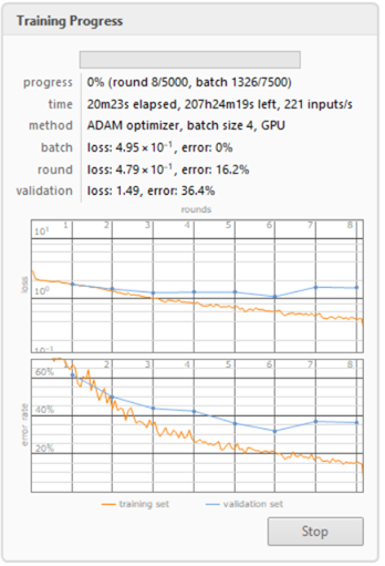
cnnTrained=NetTrain[instrumentNet,trainSet,ValidationSet->testSet,MaxTrainingRounds->5000,TargetDevice->"GPU"]
(* chop of output so results can be fed to RNN *)
cnnTrained=NetTake[cnnTrained,24]

CNN Training progress
RNN
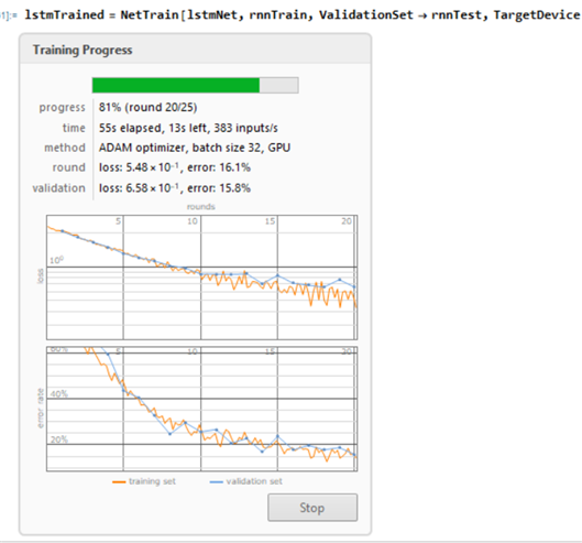
The RNN fed in the varying outputs of the CNN and outputted the genres of music. This served as a way for the computer to learn based on previous segments of a audio excerpt rather than just one long audio clip.
lstmNet=NetChain[{
LongShortTermMemoryLayer[16,"Dropout"->0.3],
LongShortTermMemoryLayer[32,"Dropout"->0.3],
SequenceLastLayer[],
LinearLayer[Length@newclasses],
SoftmaxLayer[]
},
"Input"->{"Varying",9},
"Output"->NetDecoder[{"Class",newclasses}]
]

RNN Training progress
Combining the Networks
Using both the trained networks, I created a final network which achieved an 85% accuracy.
  netCombined=NetChain[{
    NetMapOperator[cnnTrained],
    lstmTrained
    }]
(* Testing accuracy *)
cm=ClassifierMeasurements[netCombined,resizedRnnData[[900;;]],TargetDevice->"GPU"]
cm["Accuracy"]
0.8514851485148515`
Conclusion
Ultimately, the results of my project show that it is very possible to classify music accurately using machine learning. With 85% accuracy on 9 genres I think it is possible to get much higher accuracy with longer training time and more data. I plan to train the neural net on more genres with a better dataset for better recognition. For instance I would add genres such as electronic, rap, and RnB. I also plan to add multi -genre classification since many modern songs fall under multiple genres.
Cloud Deploy
First, I added the neural network to the cloud, so it could be imported as a cloud object.
CopyFile["C:\\Users\\nikhil\\Documents\\finalnet.wlnet",
 CloudObject["finalnet.wlnet"]]
Function for testing
I then created a function which partitions audio into 41 sections and mapped the net encoder onto them to convert the files into mel spectrograms. These mel spectrograms (stored as matrices) are then able to be inputted into the neural network and classified.
testFunction[audio_] := Module[{c},
  c = Import[
    CloudObject[
     "https://www.wolframcloud.com/objects/nikgad123/finalnet.wlnet"],
     "wlnet"];
  ReverseSort[
   c[Transpose[{Partition[
       NetEncoder[{"AudioMelSpectrogram", "WindowSize" -> 4096,
          "Offset" -> 1024, "SampleRate" -> 44100,
          "MinimumFrequency" -> 1, "MaximumFrequency" -> 22050,
          "NumberOfFilters" -> 128}] [audio], 41]}, {2, 1, 3, 4}],
    "Probabilities"]]


  ]

output[audio_] := Module[{str, probabilities},
  probabilities = testFunction[audio];
  str = "The predicted genre is: " <> (Keys@probabilities)[[1]] <>
    "\n" <> "\n" <> "\n";
  Column[{str,

    BarChart[probabilities, ChartLabels -> Keys@probabilities,
     LabelingFunction -> (Placed[Row[{SetPrecision[#*100, 4], "%"}],
         Above] &), ImageSize -> Large]

    }

   ]]
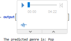
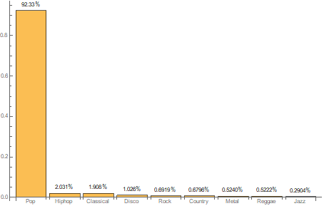
Results of the output function on Drake's Nice For What
Microsite
CloudDeploy[
 FormFunction[{"audio" -> "Sound"}, output[Audio[#audio]] &,
  AppearanceRules -> <|
    "Title" -> "Classifying Music By Genre Using Neural Networks",
    "Description" ->
     "By: Nikhil Gaddam <br> Enter a music clip to classify it:",
    "SubmitLabel" -> "Classify",
    "PageTheme" -> "Black"|>], "musicClassifier",
 Permissions -> "Public"]

CloudObject["https://www.wolframcloud.com/objects/nikgad123/\
musicClassifier"]
Here is a picture of my site: 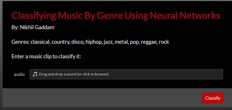
Notebook
You can download my notebook and view my computational essay and full code here: notebook download
Acknowledgments
I would like to thank my mentor Michael Kaminsky and the entire Wolfram staff for supporting me throughout the project and offering valuable advice and insight.
References