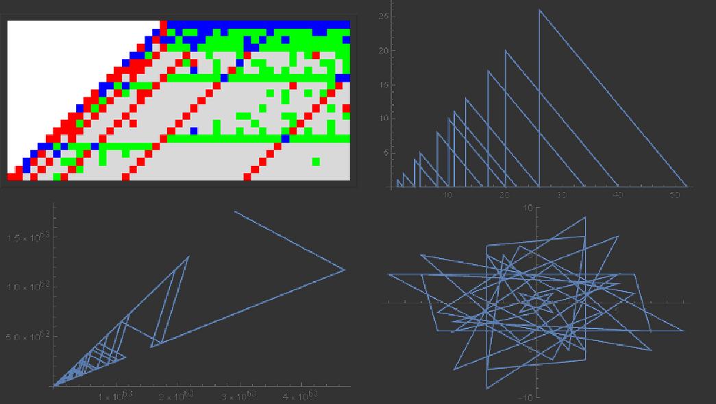
Introduction
As part of the Wolfram High School Summer Camp, I investigated the behavior of 1D and 2D generalizations of the rule for Collatz sequences (the sequences which feature in the Collatz Conjecture, also called the 3n+1 problem, among other things). A standard Collatz sequence is produced as follows: Start with any positive integer. If it is even, divide by 2. If it is odd, multiply by 3 and add 1:
$$c(n)=\left\{\begin{array}\ n/2&\text{if $n$ even}\\3n+1&\text{if $n$ odd}\end{array}\right.$$
Continue iterating this conditional. The Collatz Conjecture states that this sequence of numbers always reaches 1, regardless of the starting number. My goal was to investigate the behavior of 1D and 2D systems similar to this one.
In the end, I created numerous functions for implementing these systems, then studied them, visualizing the results that I obtained. Many of the function definitions can be found in the notebook attached to this post. I plan to continue optimizing the functions using what I have learned during the course of camp to make them faster and to produce more results.
Implementing The Standard Rule
My plan was to create functions to compute and then analyze the sequences, so I started by practicing with the case that I knew best, the original. I created a total of 8 functions (although really only 4) that allow you to investigate some of the properties of the standard Collatz sequences.
First, I created a function that simply took an integer and computed the next integer according to the rule:
CollatzStep[x_ /; IntegerQ[x] && x > 0] := If[EvenQ[x], x/2, 3 x + 1]
So, for example, 14 is even, so to find the next integer in the sequence, we divide by 2 to get 7. 7 is odd, so the next integer in the sequence after 7 is $3(7)+1=22$. This function does the same calculations, but much faster:
In[115]:= CollatzStep[14] // RepeatedTiming

Out[115]= {2.86*10^-6, 7}

In[116]:= CollatzStep[7] // RepeatedTiming

Out[116]= {2.74*10^-6, 22}
This I then used to create a second function which takes a starting integer and plots the sequence generated by that integer until it reaches 1:
CollatzPlot[x_/;IntegerQ[x]&&x>0,options:OptionsPattern[ListLinePlot]]:=
ListLinePlot[NestWhileList[CollatzStep,x,#!=1&],options]
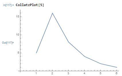
So, for example, we can plot the sequence starting with the number 5:
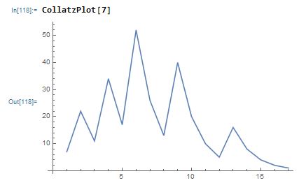
The sequence starting from 7 is much longer, notice how the shape of last peak in the sequence matches that of the sequence for 5 because the sequence for 5 is part of the sequence for 7:
CollatzPlot is extremely useful for gaining an intuition of the behavior of the Collatz sequences. Feel free to play around with it!
I then designed two other functions. CollatzResolve calculates the number of steps that it takes for the sequence to resolve to 1, while CollatzRecuce calculates the number of steps that it takes for a given starting value to reduce to a number less than itself. The amount of time that different values take to resolve to 1 or reduce in magnitude produces some interesting results when graphed. Here is a graph of the number of steps that each the first 1000 number takes to reach a value lower than itself (using a shortened version of the Collatz rule which automatically divides by 2 after applying the odd rule):
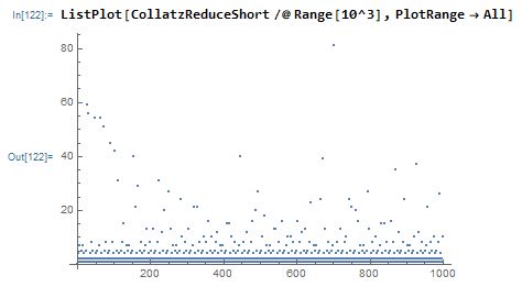
The definitions for these functions (CollatzResolve and CollatzReduce), along with some examples, are included in the notebook attached to this post. Also included are function definitions for the other 4 functions that I designed (including CollatzResolveShort, used to create the graph above), which take advantage of basic modular arithmetic to abbreviate the calculations.
Generalizing Within 1 Dimension
Functions
Having gained some practice by writing functions for the standard rule for Collatz sequences, I then turned to generalizing the functions within a single dimension. After some consideration, I decided to generalize by replacing the 3 and the 1 in the standard rule by arbitrary constants. This is a simplified version of the step function (for the full definition, see the attachment):
HailstoneStep[variable_?EvenQ,coefficient_,constant_]:=variable/2
HailstoneStep[variable_,coefficient_,constant_]:=coefficient(variable)+constant
Thus HailstoneStep[x,3,1] is equivalent to CollatzStep[x]. Then I defined a function to plot a given starting value using a given coefficient and constant for the odd rule for a specified number of steps. For example, this graphs the sequence starting with 34, which computes $11n+5$ when $n$ is odd, for 10 steps:
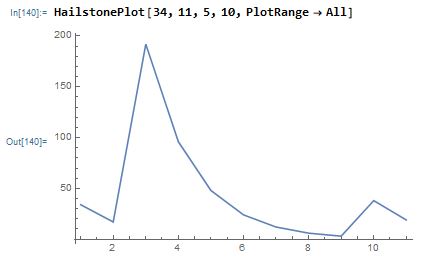
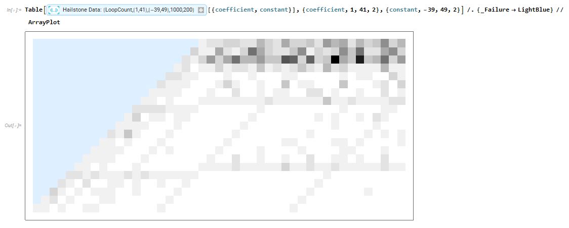
This was followed by a series of functions--one to find a loop given a specific starting value, one to find loops that arise from the first n starting values, and one to find loops in a given set of functions--that eventually built up to a function to perform an overall analysis of functions and arrange it into an association. In the end, I tested hailstone sequences of the form $$h(n)=\left\{\begin{array}\ n/2&\text{if $n$ even}\\an+b&\text{if $n$ odd}\end{array}\right.$$ where $-39\le a\le49$ and $1\le b\le39$ are odd integers, with $b$ greater than $-a$. I tested all starting values from 1 through 1000, running each for 200 steps or until I found a loop. After running the calculations in discrete packages, I combined them into an association taking the pair of values { $a$,$b$} (where $a,b$ are as defined above) to list of all of the loops that were found for that rule. I was then able to perform further analysis on the results.
Visualizations and Results
From the raw data of which loops I found for each rule, I made several visualizations.
Here is an ArrayPlot of the number of loops found for each rule. The darkest squares (where the most loops were found) occur in the row corresponding to rules of the form $5n+b$.
Here is an ArrayPlot that assigns different colors depending on the types of loops found. Rules with no loops are colored LightGray, Those with a loop including the number 1, but no others, are colored Red. Rules that have loops but do not have a known loop involving 1 are colored Green, and Rules that have both a loop involving 1 and loops not involving 1 are colored Blue.
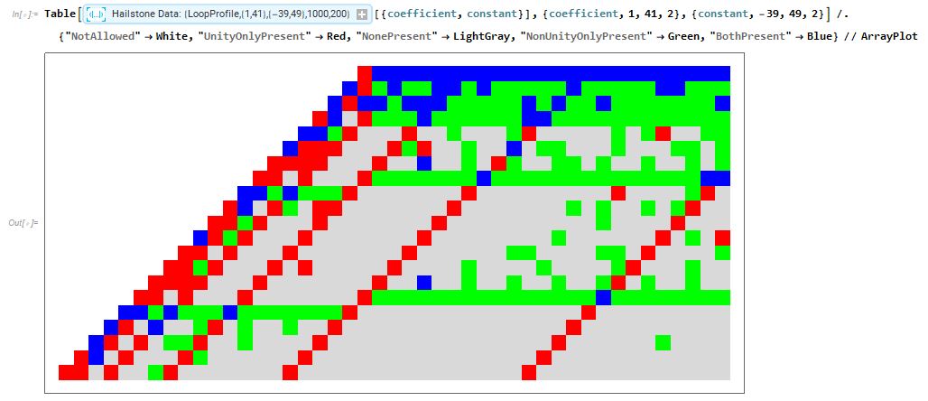
The red diagonals correspond to rules which produce powers of two directly from the number 1, such as $13n+3$, which becomes 16 for $n=1$. The green lines running across the center of the array are an unexpected finding. They correspond to rules of the form $15n+b$, $17n-b$, $31n+b$, and $33n-b$ for positive odd integer values of $b$. I hope to investigate this phenomena more closely when I have more data.
Here are some quick results about the loops that were found:
- The rule for which the most loops were found was $5n+33$, for which I found 18 loops.
- The longest loop found occurs for the rule $5n+37$ (for which 4 loops in total were found) and has length 68 (using an abbreviated version of the rule which automatically divides by 2 after computing $5n+37$).
- The largest number found which occurs in a loop is 1,601,536, which occurs for the rule $19n+33$.
Generalizing to 2 Dimensions
After my successful generalization of Collatz sequences within 1 dimension, I now started working on finding appropriate 2D analogues. Trying different rules resulted in two rules that I felt produced interesting behavior. Visualizations of both are presented here.
Rule 1:
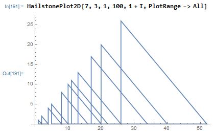
Rule 1 was defined as, for $u\in\{1,i,-1,-i\}$, $a,b\not\equiv0\mod1+i$,
$$c(n)=\left\{\begin{array}\ \overline{un/(1+i)}&\text{if }n\equiv0\mod1+i\\an+b&\text{if }n\not\equiv0\mod1+i\end{array}\right.$$
This rule is nice because setting $u=1,a=3,b=1$ reproduces the original Collatz sequence:
But the rule also can create other loops:
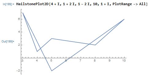
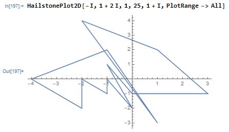
Or it can not loop:
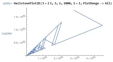
Rule 2:
Rule 2 was defined as, for $u\in\{1,i,-1,-i\}$, $a,b\not\equiv0\mod1+i$,
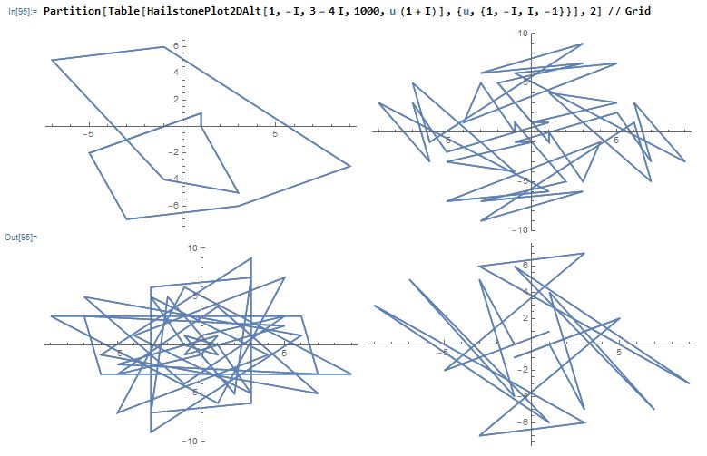
$$h(n)=\left\{\begin{array}\ un/(1+i)&\text{if }n\equiv0\mod1+i\\an+b(n\!\!\!\!\!\mod1+i)&\text{if }n\not\equiv0\mod1+i\end{array}\right.$$
where $n\mod1+i$ is computed as what the Wolfram Language gives for Mod[n,1+i]. The behavior of the latter function is not as easy to understand, and I haven't found a way to implement the original sequence with this rule, which I don't like, but it also produces very nice graphs. Here are the four graphs that you get by starting with $n=1$, $a=3$, $b=1$, and toggling the value of $u$:
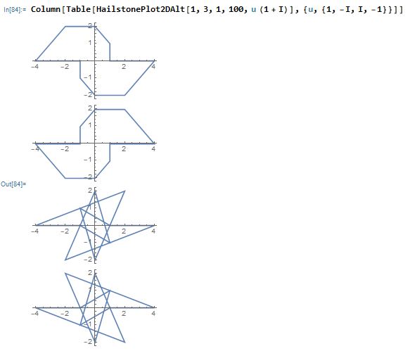
You can get these graphs by starting with $n=1,a=-i,b=3-4i$ and toggling the values of $u$:
Future Work
I plan to use the experience and knowledge that I gained during this camp to further pursue the analytical component of this project, and to see what results I can glean about generalizations of the Collatz conjecture. I will also put more study into the 2D cases, to determine what the most interesting 2D generalizations are.
Acknowledgements
Thank you to all of the mentors and instructors--Douglas, Dariia, Rick, Rob, Michael, Katie, Andrea, and Christian--for teaching me the Wolfram Language, especially when I pestered them about completely unnecessary things, and particular thanks to my mentor Chip Hurst for also acting as a sounding-board for my ideas. Thank you to Dr. Stephen Wolfram for starting the Wolfram Summer Camp and being present to answer questions and pass on his knowledge to the students, and to the admissions committee for providing financial aid so that I could attend.
 Attachments: