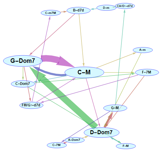
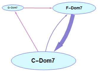
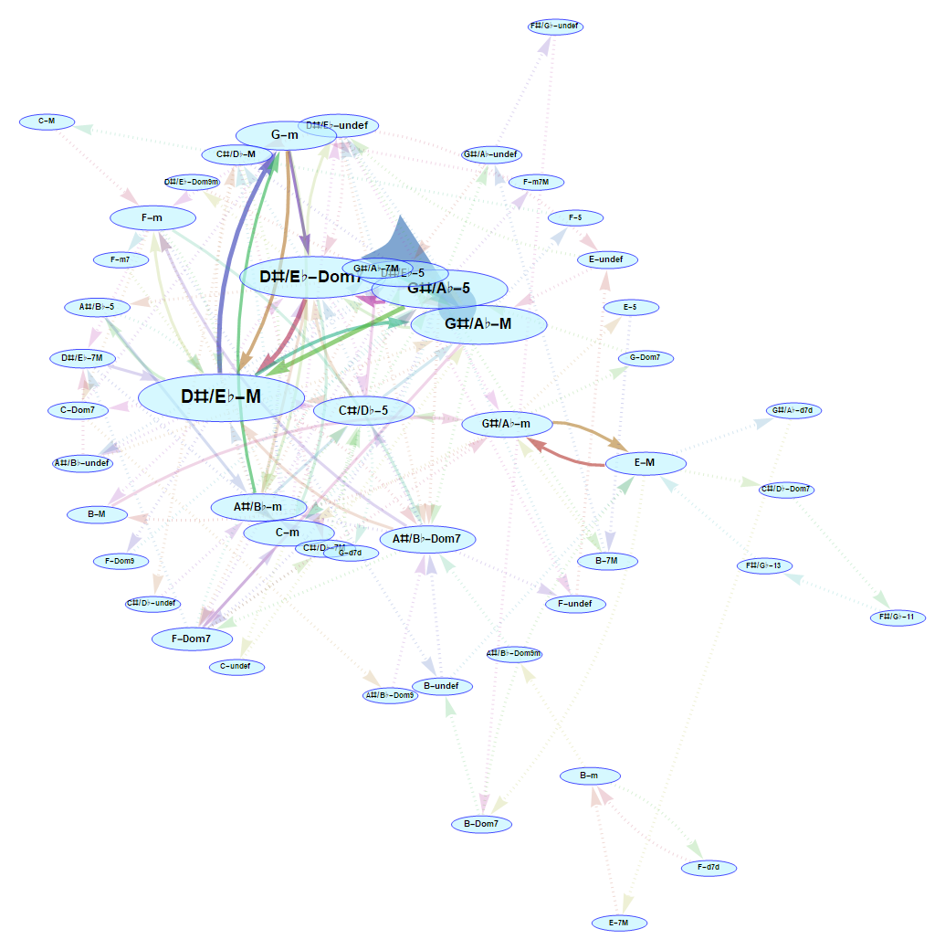
During this year's Wolfram Summer Camp, being mentored by Christian Pasquel, I developed a tool that identifies chord sequences in music (from MIDI files) and generates a corresponding graph. The graph represents all [unique] chords as vertices, and connects every pair of chronologically subsequent chords with a directed edge. Here is an example of a graph I generated:
Below is a detailed account on the development and current state of the project, plus some background on the corresponding musical theory notions.
Introduction
GOAL | The aim of this project is to develop a utility that identifies chords (e.g. C Major, A minor, G7, etc.) from MIDI files, in chronological order, and then generates a graph for visualizing that chord sequence. In the graph, each vertex would represent a unique chord, and each pair chronologically adjacent chords would be connected by a directed edge (i.e. an arrow). So, for example, if at some point in the music that is being analyzed there is a transition from a major G chord to a major C chord, there would be an arrow that goes from the G Major chord to the C Major chord. Therefore, the graph would describe a Markov chain for the chords. The purpose of the graph is to visualize frequent chord sequences and progressions within a certain piece of music.
MOTIVATION | While brainstorming for project ideas, I don't know why, I had a desire to do something with graphs. Then I asked myself, "What are graphs good at modelling?". I mentally browsed through my areas of interest, searching for any that matched that requirement. One of my main interests is music; I am somewhat of a musician myself. And, in fact, [musical] harmony is a good subject to be modelled by graphs. Harmony, one of the fundamental pillars of music (and perhaps the most important), not only involves the chords themselves, but, more significantly, the transitions between those, which is what gives character to music. And directed graphs, and, specifically, Markov models, are a perfect match for transitions between states.
Some background
Skip this if you aren't interested in the musical theory part or if you already have a background in music theory!
What is a chord?
A chord is basically a group of notes played together (contemporarily). Chords are the quanta of musical "feeling"; the typicalbut somewhat naïveexample is the sensation of major chords sounding "happy" and minor chords sounding "sad" or melancholic (more on types of chords later).
Types of chords are defined by the intervals (distance in pitch) between the notes. The root of a chord is the "most important" or fundamental note of the cord, in the sense that it is the "base" from which the aforementioned intervals are measured. In other words, the archetype of chord defines the "feel" and the general harmonic properties of the chord, while the root defines the pitch of the chord. So a "C Major" chord is a chord with archetype "major triad" (more on that later) built on the note C; i.e., its root is C.
The sequence of chords in a piece constitutes its harmony, and it can convey much more complex musical messages or feelings than a single chord, just as in language: a single word does have meaning, but a sentence can have a much more complex meaning than any single word.
Patterns in chord sequences
The main difference that between language and music is that language, in general, has a much stricter structure (i.e. the order of words, a.k.a. syntax) than music: the latter is an art, and there are no predetermined rules to follow. But humans [have a tendency to] like patterns, and music wouldn't be so universally beloved if it didn't contain any patterns. This also explains the unpopularity of atonal music (example here). But even atonal music has patterns: it may do its best to avoid harmonic patterns, but it still contains some level of rythmic, textural or other kinds of patterns.
This is why using graphs to visualize chord sequences is interesting: it is a semidirect way of identifying the harmonic patterns that distinguish different genres, styles, forms, pieces or even fragments of music. In my project, I have mainly focused on the "western" conception of tonal music, an particularly in its "classical" version (what I mean by "classical" is, in lack of a better definition, a classification that encompasses all music where the composer is, culturally, the most important artist). That doesn't mean this tool isn't apt for other types of music; it just means it will analyze it from this specific standpoint.
In tonal music, the harmonic patterns are all related to a certain notion of "center of gravity": the tonic, which is, in some way the music's harmonic "home". Classical (as in pre-XX-century) tonal music usually ends (and often starts) with the tonic chord. In fact, we can further extend the analogy with gravity by saying that music consists in a game of tension, in which the closer you are to the center of gravity (the tonic), the greater the "pull". In an oversimplified manner, the musical equivalent of the Schwarzschild radius is the dominant chord: it tends towards the tonic. Well, not really, because you can turn back from itand in fact a lot of interesting harmonical sequences consist in doing just that.
Some types of chords
In "classical" music (see definition above), there are mainly these kinds of chords (based on the amount of unique notes they contain): triad chords (i.e. three-note chords), seventh chords (i.e. four-note chords; we'll see why they're called seventh in a bit), and ninth chords (five-note chords). There is another main distinction: major and minor chords (i.e. the cliché "happy" vs "sad" distinction).
Triad chords
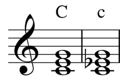
Probably the most simple and frequent chord is the triad chord (either major or minor). Here is a picture of a major and a minor triad C chord (left to right):
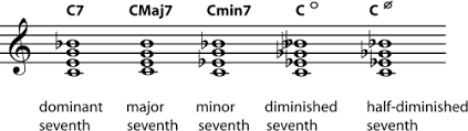
Seventh chords
Seventh chords are called so because they contain a seventh interval. Their main significance is in dominant chords, where they usually appear in the major-triad-minor-seventh (a.k.a "dominant") form. Another important seventh chord form is the fully diminished seventh chord (these will be relevant for the code later), which also tends to resolve ("resolve" is music jargon for "transition to a chord with less tension") to tonic.
Ninth chords
Although not extremely frequent, they do appear in classical music. The most "popular" is the dominant ninth chord (an extension of the dominant 7th). An alternative for this chord is the minor ninth dominant chord (built from the same dominant 7th chord, but with a minor ninth instead).
Algorithms and Code
In this section I'm going to walk through my code in order of execution. Four main parts can be distinguished in my project: importing and preprocessing, splitting the note sequence into "chunks" to be analyzed as chords, identifying the chord in each of those chunks, and visualizing the whole sequence as a graph.
First phase: importing and preprocessing the MIDI file
The first operation that needs to be done is importing the MIDI file and preprocessing it. This includes selecting which elements to import from the file, converting them to a given simplified form, and performing any sorting, deletion of superfluous elements, or other modification that needs to be done.
For this purpose I defined the function importMIDI:
importMIDI[filename_String] := MapAt[Flatten[#, 1] &, MapAt[flattenAndSortSoundNotes,
       Import[(dir <> filename <> ".mid"), {{"SoundNotes", "Metadata"}}],
1], 2]
Here dir stands for the directory where I saved all my MIDIs (to avoid having to type in the whole directory every time). Notice that we're importing the music as SoundNotes and the file's metadatawe will need it for determining the boundaries of measures (see below). The function flattenAndSortNotes does what it sound like: it converts the list of SoundNotes that Import returned into a flattened list of notes (i.e. a single track), sorted by their starting time. It also gets rid of anything that isn't necessary for chord identification (i.e. rhythmic sounds or effects). Consult the attached notebook for the explicit definition.
Here is the format the sequence of notes is returned in (i.e. importMIDI[...][[1]]):
{{"C4", {0., 1.4625}}, {"E4", {0.18125, 1.4625}}, {"G4", {0.36875, 0.525}}, <<562>>, {"G2", {105., 107.963}}, {"G4", {105., 107.963}}}
Each sub-list represents a note. Its first element is the actual pitch; the second is a list that represents the timespan (i.e. start and end time in seconds).
Second phase: splitting the note sequence into chunks
The challenge in this part of the project is knowing how to determine which notes form a single chord; i.e., where to put the boundary between one chord and the next.
The solution I came up with is not optimal, but, until now, nothing better has occurred to me (suggestions are welcome!). It involves determining where each measure start/end lies in time from the metadata and splitting each of those into a certain amount of sub-parts; then the notes are grouped by the specific sub-part of the specific measure they pertain to. The rationale behind this is that chords in classical music tend to be well-contained within measures or rational fractions of these.
This procedure is contained in the function chordSequenceAnalyzeUsingMeasures. I'm going to go over it quickly:
chordSequenceUsingMeasures[midiData_List /; Length@midiData == 2,
  measureSplit_: 2, analyzer_String: "Heuristic"] :=
 Block[{noteSequence, metadata,  chunkKeyframes, chunkedSequence,
   result},


  (*Separate notes from metadata*)
  noteSequence = midiData[[1]];
  metadata = midiData[[2]];
Until here it's pretty self evident.
  (*Get measure keyframes*)
  chunkKeyframes =
   divideByN[
    measureKeyframesFromMetadata[
     metadata, (Last@noteSequence)[[2, 2]]], measureSplit];
Here the function measureKeyframesFromMetadata is called. It fetches all of the TimeSignature and SetTempo tags in the metadata and identifies the position of each measure from them. divideByN subdivides each measure by measureSplit (an optional argument with default value 2).
  (*Chunk sequence*)
  chunkedSequence = {};
  Module[{i = 1},
   Do[
    With[{k0 = chunkKeyframes[[j]], k1 = chunkKeyframes[[j + 1]]},
     Module[{chunk = {}},
      While[
       i <= Length@noteSequence && (
         k0 <= noteSequence[[i, 2, 1]] < k1 ||
          k0 < noteSequence[[i, 2, 2]] <= k1 ),
       AppendTo[chunk, noteSequence[[i]]] i++;];
      AppendTo[chunkedSequence, chunk]
      ]
     ],
    {j, Length@chunkKeyframes - 1}]];
  chunkedSequence =
   DeleteCases[chunkedSequence, l_List /; Length@l == 0];
Once the measures' timespan has been determined, a list of "chunks" (lists of notes grouped by measure part) is generated.
  (*Call analyzer*)
  Switch[analyzer,
   "Deterministic", result = chordChunkAnalyze /@ chunkedSequence,
   "Heuristic",
   result = heuristicChordAnalyze /@ justPitch /@ chunkedSequence
   ];

  result = resolveDiminished7th[Split[result][[All, 1]]]
  ]
Finally, each chunk is sent to the chord analyzer function heuristicChordAnalyze, which I'll talk about in the next section, along with the currently mysterious resolveDiminished7th.
Since this algorithm for "chunking" a note sequence doesn't work for everything, I also developed an alternative, more naïve approach:
chordSequenceNaïve[midiData_List /; Length@midiData == 2,
  analyzer_String: "Heuristic", n1_Integer: 6, n2_Integer: 1] :=
 Module[{noteSequence, chunkedSequence, result},

  (*Separate notes from metadata*)
  noteSequence = midiData[[1]];

  (*Chunk sequence*)
  chunkedSequence = Partition[noteSequence, n1, n2];

  (*Call analyzer*)
  result = heuristicChordAnalyze /@ justPitch@chunkedSequence;

  result = resolveDiminished7th[Split[result][[All, 1]]]
  ]
Phase 3: identifying the chord from a group of notes
This has been the main conceptual challenge in the whole project. After some unsucsessful ideas, with some suggestions from Rob Morris (one of the mentors), whom I thank, I ended up developing the following algorithm. It iterates through each note and assigns it a score that represents the likeliness of that note being the root of the chord based on the presence of certain indicators (i.e. notes the presence of which define a chord, to some degree), each of which with a different weight: having a fifth, having a third, a minor seventh... Then the note with the highest chord is assumed to be the root of the chord.
In code:
heuristicChordAnalyze[notes_List] :=
 Block[{chordNotes, scores, root},

  (*Calls to helper functions*)
  chordNotes = octaveReduce /@ convertToSemitones /@ notes // DeleteDuplicates;

  (*Scoring*)
  scores = Table[Total@
  Pick[
   (*Score points*)
   {24, 16, 16, 8, 2, 3, 1, 1,
    10, 15, 15, 18},

   (*Conditions*)
   SubsetQ[chordNotes, #] & /@octaveReduce /@
      {{nt + 7}, {nt + 4}, {nt + 3}, {nt + 10}, {nt + 11}, {nt + 2}, {nt + 5}, {nt + 9},
      {nt + 4, nt + 10}, {nt + 3, nt + 6, nt + 10}, {nt + 3, nt + 6, nt + 9}, {nt + 1, nt + 4, nt + 10}}
   ]

     (*Substract outliers*)
     - 18*Length@Complement[chordNotes, octaveReduce /@ {nt, 7 + nt, 4 + nt, 3 + nt, 10 + nt, 11 + nt,
                                                         2 + nt, 5 + nt, 9 + nt, 6 + nt}],

   {nt, chordNotes}];

  (*Return*)
  root = Part[chordNotes, Position[scores, Max @@ scores][[1, 1]]];

  {root, Which[
    SubsetQ[chordNotes, octaveReduce /@ {root + 10 , root + 2, root + 5, root + 9}], "13",
    SubsetQ[chordNotes, octaveReduce /@ {root + 10, root + 2, root + 5}], "11",
    SubsetQ[chordNotes, octaveReduce /@ {root + 4, root + 10, root + 2}], "Dom9",
    SubsetQ[chordNotes, octaveReduce /@ {root + 4, root + 10, root + 1}], "Dom9m",
    SubsetQ[chordNotes, octaveReduce /@ {root + 11, root + 7, root + 3}], "m7M",
    SubsetQ[chordNotes, {octaveReduce[root + 11], octaveReduce[root + 4]}],  "7M",
    SubsetQ[chordNotes, {octaveReduce[root + 10], octaveReduce[root + 4]}],  "Dom7",
    SubsetQ[chordNotes, {octaveReduce[root + 10], octaveReduce[root + 7]}], "Dom7",
    SubsetQ[chordNotes, {octaveReduce[root + 10], octaveReduce[root + 6]}],  "d7",
    SubsetQ[ chordNotes, {octaveReduce[root + 9], octaveReduce[root + 6]}],  "d7d",
    SubsetQ[chordNotes, {octaveReduce[root + 10], octaveReduce[root + 3]}],  "m7",
    MemberQ[chordNotes, octaveReduce[root + 4]], "M",
    MemberQ[chordNotes, octaveReduce[root + 3]], "m",
    MemberQ[chordNotes, octaveReduce[root + 7]], "5",
    True, "undef"]}
]
A note on notation
In this project I use the following abbreviations for chord notation (they're not in the standard format). "X" represents the root of the chord.
- X-5** = undefined triad chord (just the root and the fifth)
- X-M** = Major
- X-m** = minor
- X-m7** = minor triad with minor (a.k.a dominant) seventh
- X-d7d** = fully diminished 7thchord
- X-d7** = half diminished 7thchord
- X-Dom7** = Dominant 7th chord
- X-7M** = Major triad with Major 7th
- X-m7M** = minor triad with Major 7th
- X-Dom9** = Dominant 9th chord
- X-Dom9m** = Dominant 7th chord with a minor 9th
- X-11** = 11th chord
- X-13** = 13th chord
Dealing with diminished 7th chords
Now, on to resolveDiminished7th. What is this function on about?
Well, recall the fully diminished seventh chords I mentioned in the Background section. Here's the problem: they're completely symmetrical! What I mean by that is that the intervals between subsequent notes are identical, even if you invert the chord. In other words, the distance in semitones between notes is constant (it's 3) and is a factor of 12 (distance of 12 semitones = octave). So, given one of these chords, there is no way to determine which note is the root just by analyzing the chord itself. In the context of our algorithm, every note would have the same score!
At this point I thought: "How do humans deal with this?". And I concluded that the only way to resolve this issue is to have some contextual vision (looking at the next chord, particularly), which is how humans do it. So what resolveDiminished7th does is it brushes through the chord sequence stored in result, looking for fully diminished chords (marked with the string "d7d"), and re-assigns each of those a root by looking at the next chord:
resolveDiminished7th[chordSequence_List] :=
Module[{result},
  result = Partition[chordSequence, 2, 1] /. {{nt_, "d7d"}, c2_List} :> Which[
  MemberQ[octaveReduce /@ {nt, nt + 3, nt + 6, nt + 9}, octaveReduce[c2[[1]] - 1]], {{c2[[1]] - 1, "d7d"}, c2},
  MemberQ[octaveReduce /@ {nt, nt + 3, nt + 6, nt + 9}, octaveReduce[c2[[1]] + 4]], {{c2[[1]] + 4, "d7d"}, c2},
  MemberQ[octaveReduce /@ {nt, nt + 3, nt + 6, nt + 9}, octaveReduce[c2[[1]] + 6]], {{c2[[1]] + 6, "d7d"}, c2},
  True, {{nt, "d7d"}, c2}];

result = Append[result[[All, 1]], Last[result][[2]]]
]
Phase 4: Visualization
Basically, my visualization function (visualizeChordSequence) is fundamentally a highly customized call of the Graph function; so I'll just paste the code below and then explain what some parameters do:
visualizeChords[chordSequence_List, layoutSpec_String: "Unspecified", version_String: "Full", mVSize_: "Auto", simplicitySpec_Integer: 0, normalizationSpec_String: "Softmax"] :=
 Module[{purgedChordSequence, chordList, transitionRules, weights, graphicalWeights, nOfCases, edgeStyle, vertexLabels, vertexSize, vertexStyle, vertexShapeFunction, clip},


  (*Preprocess*)
  Switch[version,
   "Full",
   purgedChordSequence =
    StringJoin[toNoteName[#1], "-", #2] & @@@ chordSequence,
   "Basic",
   purgedChordSequence =
    Split[toNoteName /@ chordSequence[[All, 1]]][[All, 1]]];


  (*Amount of each chord*)
  chordList = DeleteDuplicates[purgedChordSequence];
  nOfCases = Table[{c, Count[purgedChordSequence, c]}, {c, chordList}];

  (*Transition rules between chords*)
  Switch[version,
   "Full",
   transitionRules =
    Gather[Rule @@@ Partition[purgedChordSequence, 2, 1]],
   "Basic",
   transitionRules =(*DeleteCases[*)
    Gather[Rule @@@ Partition[purgedChordSequence, 2, 1]](*, t_/;
   Length@t\[LessEqual]2]*) ];


  (*Get processed weight for each transition*)
  weights = Length /@ transitionRules;
  If[normalizationSpec == "Softmax", graphicalWeights = SoftmaxLayer[][weights]];;
  graphicalWeights =
   If[Min@graphicalWeights != Max@graphicalWeights,
    Rescale[graphicalWeights,
     MinMax@graphicalWeights, {0.003, 0.04}],
    graphicalWeights /. _?NumericQ :> 0.03 ];

  (*Final transition list*)
  transitionRules = transitionRules[[All, 1]];

  (*Graph display specs*)
  clip = RankedMax[weights, 4];

  edgeStyle =
   Table[(transitionRules[[i]]) ->
     Directive[Thickness[graphicalWeights[[i]]],
      Arrowheads[2.5 graphicalWeights[[i]] + 0.015],
      Opacity[Which[
        weights[[i]] <= Clip[simplicitySpec - 2, {0, clip - 2}], 0,
        weights[[i]] <= Clip[simplicitySpec, {0, clip}], 0.2,
        True, 0.6]],
        RandomColor[Hue[_, 0.75, 0.7]],
      Sequence @@ If[weights[[i]] <= Clip[simplicitySpec - 1, {0, clip - 1}], {
         Dotted}, {}] ], {i, Length@transitionRules}];

  vertexLabels =
   Thread[nOfCases[[All,
      1]] -> (Placed[#,
         Center] & /@ (Style[#[[1]], Bold,
           Rescale[#[[2]], MinMax[nOfCases[[All, 2]]],
            Switch[mVSize, "Auto", {6, 20}, _List,
             10*mVSize[[1]]/0.3*{1, mVSize[[2]]/mVSize[[1]]}]]] & /@
         nOfCases))];

  vertexSize =
   Thread[nOfCases[[All, 1]] ->
     Rescale[nOfCases[[All, 2]], MinMax[nOfCases[[All, 2]]],
      Switch[mVSize,
       "Auto", (Floor[Length@chordList/10] + 1)*{0.1, 0.3}, _List,
       mVSize]]];

  vertexStyle =
   Thread[nOfCases[[All, 1]] ->
     Directive[Hue[0.53, 0.27, 1, 0.6], EdgeForm[Blue]]];

  vertexShapeFunction =
   Switch[version, "Full", Ellipsoid[#1, {3.5, 1} #3] &, "Basic",
    Ellipsoid[#1, {2, 1} #3] &];


  Graph[transitionRules,

   GraphLayout ->
    Switch[layoutSpec, "Unspecified", Automatic, _, layoutSpec],

   EdgeStyle -> edgeStyle,
   EdgeWeight -> weights,
   VertexLabels -> vertexLabels,
   VertexSize -> vertexSize,
   VertexStyle -> vertexStyle,
   VertexShapeFunction -> vertexShapeFunction,
   PerformanceGoal -> "Quality"]
  ]
There are five main things to focus on in the above definition: the graph layout (passed as the argument layoutSpec), the edge thickness (defined in edgeStyle), the vertex size (defined in vertexSize), the version (passed as argument version) and the simplicity specification (simplicitySpec).
The graph layout is a Graph option that can be specified in the argument layoutSpec. If "Unspecified" is passed, an automatic layout will be used. I find that the best layouts tend to be, in order of preference, "BalloonEmbedding" and "RadialEmbedding"; nevertheless, neither are a perfect fit for every piece. In the future I would like to to implement custom (i.e. pre-defined) positioning, so that I can design it in a way that best fits this project.
The edge thickness is a function of the amount of times a certain transition between two chords has occurred in the chord sequence. There is an option (namely the normalizationSpec argument) to enable or disable using a Softmax function for assigning thicknesses to edges. This is due to the fact that for simple/short chord sequences, Softmax is actually counterproductive because it suppresses secondary but still top-ranked transitions; i.e., it assigns a very high thickness to the most frequent transition and a low thickness to all other transitions (even those that come in second or third in frequency ranking). But for large or complex sequences it is actually useful, because it "gets rid of" a lot of the [relatively] insignificant instances, thus making the output actually understandable (and not just a jumbled mess of thick lines).
The vertex size is proportional to the number of occurrences of each particular chord (that is, without taking into account the transitions). It can also be specified manually by passing vSize as a list {a,b} such that a is the minimum size an b is the maximum.
The version can be either "Full" or "Basic"; the default is "Full". The "Basic" version consists of a simplified chord set in which only the root note of the chord is taken into account, and not the archetype. For example, all C chords (M, Dom7, m...) would be represented by a single "C" vertex.
Finally, the simplicity specification (simplicitySpec) is a number that can be thought of, in some way, as a "noise" threshold: as it gets larger, fewer edges "stand out"that is, more of the lower-significance ones are rendered with reduced opacity or are shown as dotted lines. This is useful for large or complex sequences.
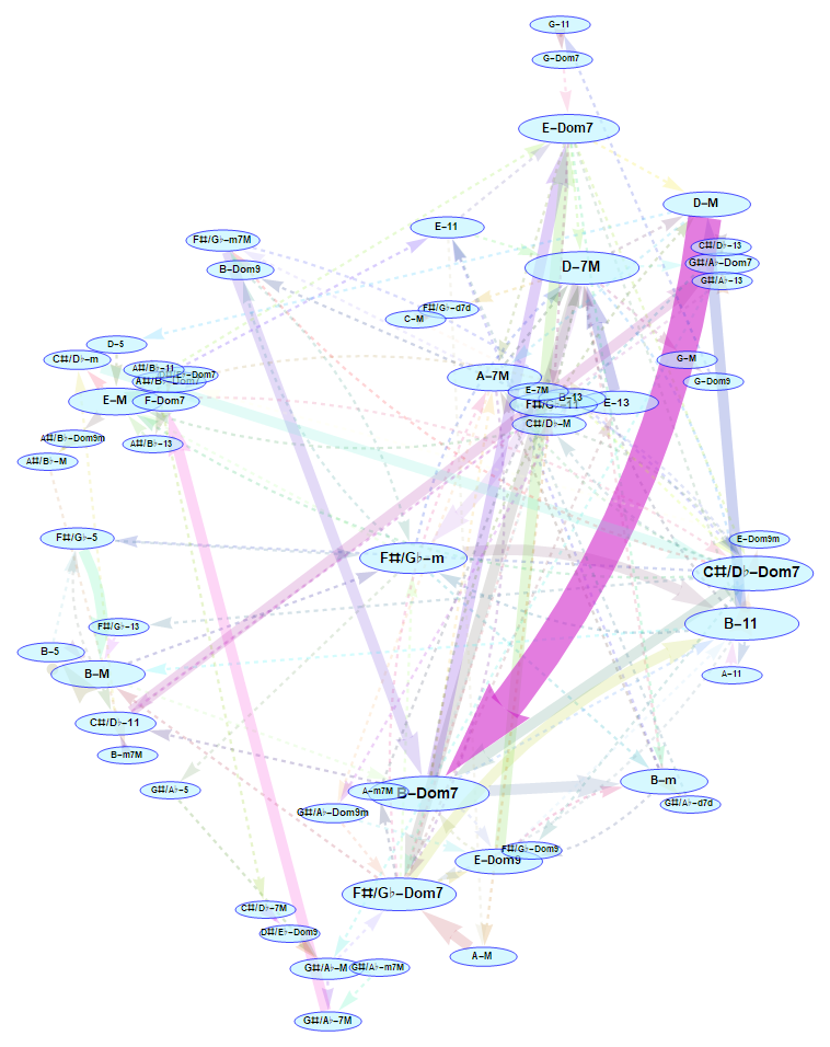
Some examples
Here I will show some specific examples generated with this tool. I tried to use different styles of music for comparison.
- Debussy's Passepied from the Suite Bergamasque:
- A "template" blues progression:
- Beethoven's second movement from the Pathétique sonata (no.8):
- Any "reggaeton" song (e.g. Despacito):

Microsite
Check out the form page (a.k.a. microsite) of this project here:
https://www.wolframcloud.com/objects/lammenspaolo/Chord%20sequence%20visualization
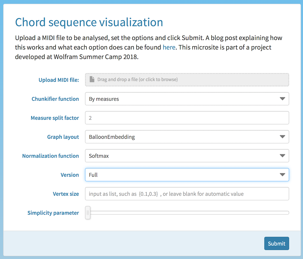
Briefly, here is what each option does (see the section Algorithms and code for a more detailed explanation):
- Chunkifier funciton: choose between splitting notes by measures or by a constant amount of notes
- Measure split factor: choose into how many pieces you want to divide measures (each piece will be analyzed as a separate chord)
- Graph layout: choose the layout option for the
Graph call
- Normalization function: choose whether to apply a Softmax function to the weights of edges (to make results clearer in case of complex sequences).
- Version: choose "Full" for complete chord info (e.g. "C-M", "D-Dom7", "C-7M"...) or "Basic" for just the root of the chord (e.g. "C", "D"...)
- Vertex size: specify vertex size as a list
{a,b} where a is the minimum and b is the maximum size
- Simplicity parameter: visual simplification of the graph (a value of 0 means no simplification is applied)
Conclusions
I have developed a functional tool to visualize chord sequences as graphs. It is far from perfect, though. In the future, I would like improving the positioning of vertices, being able to eliminate insignificant transitions from the graph altogether, and making other visual adjustments. Furthermore, I plan to refine and optimize the chord analyzer, as right now it is just an experimental version that isn't too accurate. A better "chunkifier" function could be developed too.
Finally, I'd like to thank my mentor Christian Pasquel and all of the other WSC staff for this amazing opportunity. I'd also like to thank my music theory teacher, Raimon Romaní, for making me, over the years, sufficiently less terrible at musical analysis to be able to undertake this project.
 Attachments:


