Introduction
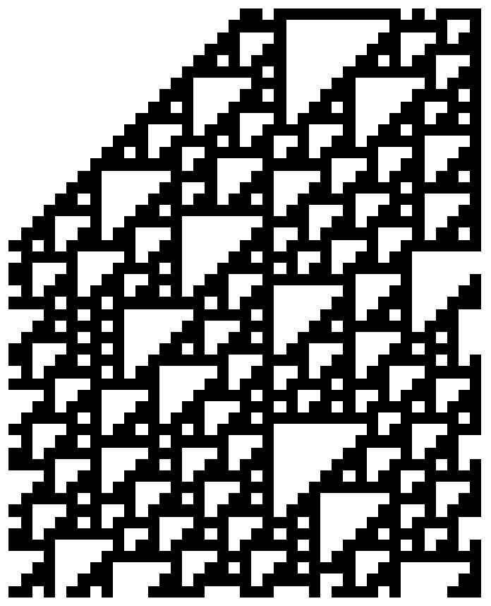
I worked on figuring out a way to computationally locate and identify gliders in cellular automaton(CA). More specifically, my research was contained to one rule in CA: rule 110. The goal was to analyze this rule and create a "panning window" across an arbitrary cellular structure that would return the identification of the glider. This goal may prompt one to ask the questions: what purpose does cellular automaton serve and why is identifying gliders important? In Stephen Wolfram's A New Kind of Science he explores the derivation, analysis, and application of these structures. He goes into depth on the modeling power CAs hold, from the second law of thermodynamics to being able to find prime integers, CA structures offer a new way to think and approach complex mathematical and physical principles. One of the most noteworthy examples Wolfram provides his readers is his use of CAs to think deeper about the fundamental constructs of the universe. Postulating that at infinitesimal distances the universe may be made up of smaller fragments similar to the constructs we observe in CAs. A major theme --often discussed in A New Kind of Science--to consider while reading my project is that while traditional mathematics and physics may predict a continuous structure or smooth surface it may be at a infinitesimal scale be made up of discrete smaller patterns that only appear to be smooth in nature. By formulating ways to effectively analyze CAs we can begin to answer questions that before seemed impossible.
Heuristic Approach
Transposing an array to search for long strands of ones and zeros
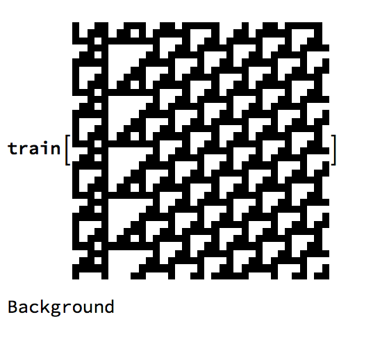
The simplicity of the rules that govern CAs tempted me to explore a heuristic approach. Using the Wolfram Research Data Repository, Stephen Wolfram had conveniently posted the 16 local persistent structures that appear in rule 110. It is important to keep in mind that while CA structures are complex, to the computer the structure is a mere matrix of 1's and 0's. Some code and structures are shown below
CellularAutomaton[110,Join[Table[RandomInteger[0], 20], {1}, Table[RandomInteger[1], 20]], 50];

First thoughts made me take a complex cellular structure and rotate the structure an x number of moves to the right or to the left. In theroy if a structure had a linear repitition the now transposed array should have peaks of zeros or ones that correspond with gliders. Some code about this process is shown below.
ca = CellularAutomaton[110, Join[Table[RandomInteger[1], 8], {1}, Table[RandomInteger[1], 8]], 25];
rowDataRight = Table[RotateRight[ca[[n]], (n - 1)], {n, 1, Length[ca]}];
rowDataLeft = Table[RotateLeft[ca[[n]], (n - 1)], {n, 1, Length[ca]}];
Row[{ArrayPlot[ca], Column[ca], Column[rowDataRight], Column[rowDataLeft]}]
Here the output has 4 items: the actual cellular structure, the matrix of that structure, the matrix rotated to the right by 1, the matrix roared to the left by 1
Because the background of the rule 110 structure is of length 14 and rereats every 7 steps and also is made up of a linear step patten this method does not identify where gliders are but where there are an absence of gliders and a continous area of just background structures.
Accounting for the pattern, pattern length and its position in the structure.
I then attempted to satisfy three conditions: length, pattern and position. For each individual cellular structure I attempted to not only look for the repeating strucure but present the length and position of where the pattern occured in a readable way. This strategy transversed a section of the matrix of the pattern occuring and also mapped the row that it occured in. It would be intuitve that if one looked a number of steps down and number of shifts over that the same patten would occur an x amount of times until the glider had a collision or died out. Here is how I extracted the single glider images from the data repository to test this heuristic.
With[{
  bkg = ResourceData["Persistent Structures in Rule 110", All]["Background"],
  structs = Normal@ResourceData["Persistent Structures in Rule 110"]},
  ArrayPlot[
    CellularAutomaton[110,
     Flatten[{Table[bkg, 8], #Cells, Flatten[Table[bkg, 8]]}], 250],
    ImageSize -> {Automatic, 300}, PixelConstrained -> 1] & /@
  Take[structs, 16]]
By storing the data from one cellular structure into an arbitrary variable cellData we can begin to look and map out the exact positions of certain strands of ones and zeros that are unique to the structure. You could do this by implementing the following:
Rest@PositionIndex[Flatten[SequencePosition[#, {0, 1, 0, 1, 1, 1, 0}]] & /@ celldata]
This specific snippet of code transverses the array to look for the strand of zeros and ones: {0,1,0,1,1,1,0}. An example output for a moderately sized CA is shown below.

While this method can very eaily identify a simple structure that only contains one structure, when applied to a CA that has a more complex structure its unreasonable to transerve the array for every shift, period, and pattern for of all sixteen local persistant structures in rule 110. The main problem with this method was the appearence of the structure in other places, where gliders to do exist. Even if one were able to find the pattern at the right length and repition sometimes the addition of the background and the glider make it seem as though you have found the glider while actually you havent found anytning. This also seemed too computionally intensive as the most likely strategy to solve this problem.
Artifical Intellingence Approach
Getting the Data Set
To get a viable data set I extracted Stephen Wolfram's data repository on persiatnant structures in rule 110 where he gives the 16 different gliders that occur. Unforunatly with machince learning it's impossible to train a Machine Learning Algorithm with a dataset of 16. Using the code provided in the repository I was able to apply ImagePartition to the structure and apply an algorithm that when given a prestructure of a glider, an image partition size, and threshold to return only images of gliders, not the background.
findStructures[prestructure_, fragmentsize_, thres_Real] :=
  Module[{flatstructure, backgroundbig, backgrounds, structure, onz}, structure =  ImageCrop[ prestructure, {ImageDimensions[prestructure][[1]] - 4,
  ImageDimensions[prestructure][[2]] - 4}];
   backgroundbig = Rasterize[ArrayPlot[ CellularAutomaton[110, Flatten[Table[
   ResourceData["Persistent Structures in Rule 110", All] ["Background"], Round[fragmentsize/14] + 10]],
   fragmentsize + 140], PixelConstrained -> 1, PlotRangePadding -> 0]];
   backgrounds = Table[ImagePartition[ImageCrop[backgroundbig, {fragmentsize + 138 - 2 n,
  fragmentsize + 136}], fragmentsize][[1, 1]], {n, 0, 13}];
   structureQ[pic_] := Min[Table[
   ImageMeasurements[ImageSubtract[pic, backgrounds[[q]]],
   "Mean"][[1]], {q, 1, 14}]];
   flatstructure = Flatten[ImagePartition[structure, fragmentsize]];
   onz = Table[structureQ[flatstructure[[n]]], {n, 1, Length[flatstructure]}];
   DeleteCases[Table[If[onz[[n]] > thres, flatstructure[[n]], ""], {n, 1,
    Length[flatstructure]}], ""]];
structurecheckList[list_List, num_, thre_] := Flatten@ParallelTable[findStructures[list[[x]], num, thre], {x, 1, Length[list]}];
To get different iterations and permutations I adjusted the intial conditions to have a different length; this effectively translates the structure a very small distance to the left or to the right, but allows the image partition to be trained on a vareity of positions that the structure could have. You can loop over very small fragments to ensure the threshold still holds valid.
GliderCdata = Flatten@ParallelTable[ Image[With{
     bkg = ResourceData["Persistent Structures in Rule 110", All]["Background"],
        structs = Normal@ResourceData["Persistent Structures in Rule 110"]},
       ArrayPlot[CellularAutomaton[110, Flatten[{Table[bkg, x], #Cells, Flatten[Table[bkg, 10]]}], 260],
       ImageSize -> {Automatic, 300},
       PixelConstrained -> 1] & /@ Take[structs, {3, 3}]][[1]]], {x, 8, 80, 0.1}];
GliderCconformed = ConformImages[structurecheckList[Cd, 35, 0.235]];
When this algorithm runs over the CA a protracted result looks like the following:

From here, processing the data is simple. I simply threaded a classification through for each subset of Glider (A-O) and also made a data set for the background that appears in Rule 110. It can be found on the data repository.
Training a Neural Network
This is a very challenging step in the process of classifying gliders. Its difficult to know what artitechure will optimize the accuracy. Looking over the Wolfram Neural Network repository I wanted to find something that analyzed smaller grayscale images. The closest net to these specifications was LeNet. Making some new layers and deleting a few others we constructed this neural net.
net = NetTake[ NetModel["LeNet Trained on MNIST Data", "UninitializedEvaluationNet"], 7];
classes = {"A", "B", "C", "D", "E", "F", "G", "H", "I", "J", "K", "L", "M", "N", "O", "Background"};

finalNet = NetChain[{
   NetReplacePart[net,
    "Input" -> NetEncoder[{"Image", {40, 40}, ColorSpace -> "Grayscale"}]],
   LinearLayer[16],
   Ramp,
   LinearLayer[16],
   SoftmaxLayer[]
   },
  "Input" -> NetEncoder[{"Image", {40, 40}, ColorSpace -> "Grayscale"}],
  "Output" -> NetDecoder[{"Class", classes}]
  ]

The accuracy for this neural net on larger structure CAs got an accuracy just above 40%. We noticed the sensitivity of the program is quite large. A structure with even a pixel off from the data will cause the neural net to misidentify a glider for a background or even return the name of another glider. The confusion matrix plot revealed a misidentification of a large proportion of Gliders A and O this might be due to the fact that they're the smallest structure and the difference between the two are incredibly small. With similar data from the data set is actually found in a CA we can achieve approximately a 90 percent accuracy, but when the neural network is given larger CA structures the program's accuracy essentially dilutes down to guessing.
Deeper Learning
It's quite obvious that LeNet is a very shallow neural network and that the learning isn't very deep. Inspired by ResNet, also found on the data repository, I attempted to modify the aritecture to comply with my data set. See Below.
tempNet = Take[NetModel[ "ResNet-50 Trained on ImageNet Competition Data"], {1, -4}];
classes = {"A", "B", "C", "D", "E", "F", "G", "H", "I", "J", "K", "L", "M", "N", "O", "Background"};

 finalNet = NetChain[{
   NetReplacePart[net,
    "Input" -> NetEncoder[{"Image", {40, 40}, ColorSpace -> "Grayscale"}]],
   LinearLayer[16],
   Ramp,
   LinearLayer[16],
   SoftmaxLayer[]
   },
  "Input" -> NetEncoder[{"Image", {40, 40}, ColorSpace -> "Grayscale"}],
  "Output" -> NetDecoder[{"Class", classes}]
  ]
By upscaling the data set ResNet could anaylze it better. We achieved a higher accuracy with the specifications that were given to the neural network. But once again if the image partitions of a random CA are too large too small or a different permutation of a background the neural network's probability essentially drops to guessing, not much improvement. Here's an example of a scaled version where it makes a humorous error. 
Further Research
A lot of further reaserch can be conducted on this topic.
Is it better to give a neural network larger or smaller images? Does it "learn" better? Can we quantify this improvement and track down the fundamental reason why?
Can we train a neural network to find collisons in cellular automata?
Through exploration can we use machine learning to find gliders in other structures?
Can we use artifical intellligence to find any conservation laws in cellular automaton?
Are there more conservation laws that govern collisons in rule 110 that Stephen Wolfram has not explored? Do these conservation laws exsist in other rules or structures?
 Attachments: