This project seeks to find the shortest distance between two coordinate locations on the surface of the Earth given a maximum possible slope, or threshold. I created a function called shortestDistance that takes four parameters: the first coordinate location (or city), the second coordinate location (or city), the slope threshold, and the image resolution. Using a module, I declared all of my local variables:
    shortestDistance[c1_, c2_, quality_, threshold_] :=
    Module[{pos1, pos2, dist, bounds, br, center, geoRange, realPixelSize,
        data, terrainImage, gradient, d, m, rel, xn, yn, edges, graph, v,
        bin, del, pg, path, pix1, pix2, fullTerrain, mag, mesh, newPath,
        dropOne, testPath, scaledLength, actualLength, $size},
After that, I stored the coordinate points in {x, y} format of the two user-entered locations into the variables "pos1" and "pos2":
    pos1 = GeoPosition[c1];
    pos2 = GeoPosition[c2];
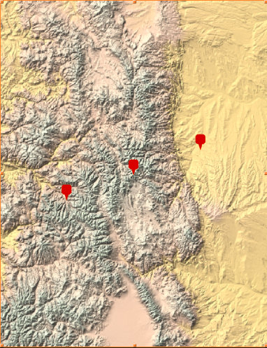
The bounds of the image were adjusted to fit the entire area of interest. In this example, c1 represents Denver, CO and c2 represents Aspen, CO, and the adjusted terrain graph is shown below with the locations of the two cities and the midpoint between the cities.
   bounds = CoordinateBounds[{pos1[[1]], pos2[[1]]}];
    br = Max[#2 - #1 & @@@ bounds];
    center = Mean[{pos1[[1]], pos2[[1]]}];
    geoRange = Transpose[{center - br, center + br}];
and the elevation data was stored as a matrix in the variable "data."
data = GeoElevationData[Transpose@geoRange];
I created four possible pixel dimensions for the size of the newly scaled image and assigned the value to the variable "$size" (eg. choice 2-> {200,200} would correspond to a 200 by 200 pixel resolution). The different resolutions were added to the menu because higher resolutions mean slower runtime: the user has the option to choose between speed and the quality of the image.
    $size = Replace[
    quality, {1 -> {50, 50}, 2 -> {200, 200}, 3 -> {300, 300},
    4 -> {400, 400}}];
Next, I created a function "pixelSize" in order to determine the real distance of the path, in miles, given the distance of the path in pixels, and the definition of the function is shown below. Here, the function takes in two arguments: the range of the pixel values for the x and y coordinates as a single list "geoRange" and a "resolution" argument representing the pixel dimensions specified by the user, which was stored in $size in the previous step.
    pixelSize[geoRange_, {resolution_, _}] :=
    Module[{x1, x2, y1, y2},
    {{x1, x2}, {y1, y2}} = geoRange;
    GeoDistance[
    GeoPosition[{x1, y1}],
    GeoPosition[{x2, y1}]
    ]/resolution
    ];
In the function call below, realPixelSize represents the ratio of $\frac{actual}{scaled}$ pixel lengths, and the original terrain image is rescaled to an image of the user-entered pixel dimensions
    realPixelSize = pixelSize[geoRange, $size];
    terrainImage = ImageResize[Image[QuantityMagnitude[data]], $size];
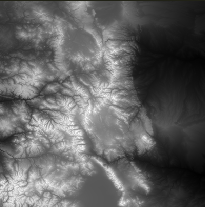
The image below represents the resized terrain image, with lighter areas representing higher elevations while darker areas representing lower elevations:
In one of the most important steps, the gradient filter is applied to the scaled terrain image:
gradient = GradientFilter[terrainImage, 1];
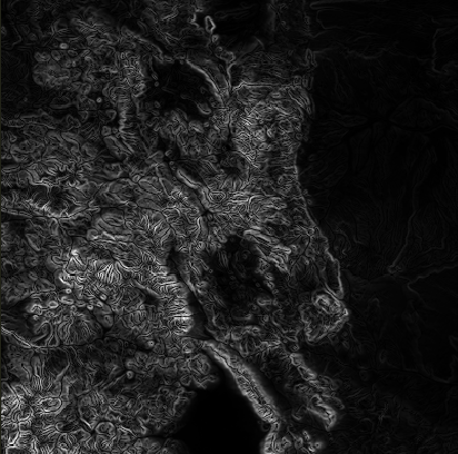
Now for the gradient image...the image is lighter in areas with greater slope (unlike elevation of the terrain image) and darker in relatively flat terrain with little to no steepness.
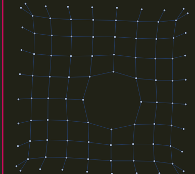
In the next block of code, each pixel on the gradient image is connected to the four adjacent pixels, and the duplicates are deleted using the DeleteDuplicates function since every two adjacent pixels (eg. pixel A and pixel B) will be connected twice (A->B and B->A) before the duplicates are deleted.
    d = #2 - #1 & @@@ geoRange;
    m = #1 & @@@ geoRange;
    rel = Round[Reverse[$size*(#[[1]] - m)/d] & /@ {pos1, pos2}];
    {xn, yn} = ImageDimensions[gradient];
    edges = DeleteDuplicatesBy[Flatten@Table[{
          Pixel[i, j] \[UndirectedEdge] Pixel[i - 1, j],
          Pixel[i, j] \[UndirectedEdge] Pixel[i + 1, j],
          Pixel[i, j] \[UndirectedEdge] Pixel[i, j - 1],
          Pixel[i, j] \[UndirectedEdge] Pixel[i, j + 1]
          }, {i, 2, xn - 1}, {j, 2, yn - 1}], Sort];
    graph = Graph[edges];
    v = VertexList[graph];
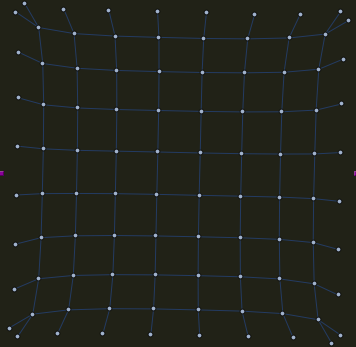
Here is a visualization of the connected pixels after duplicates are deleted.
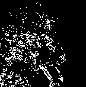
The Binarize function is now applied to the gradient image, and all the pixel values greater than the user-inputted threshold will be replaced with a white pixel while all the pixel values less than the threshold will be replaced with a black pixel. The resulting binarized image is stored in the variable "bin."
bin = Binarize[gradient, threshold];
All the white pixels (pixels with gradient above threshold) will be deleted using a separate function called FastVertexDelete, for which the definition and function call are down below:
Side Note:
Why wasn't VertexDelete, a predefined function in Mathematica, used?
VertexDelete took a long time to run, due to a possible bug in the function...to cut down runtime, a new function "FastVertexDelete" was created.
Definition of FastVertexDelete:
FastVertexDelete[ graph_Graph, delete_List ] :=
  With[ { dropQ = AssociationMap[ True &, delete ] },
      Graph[ Complement[ VertexList @ graph, delete ],
             DeleteCases[ EdgeList @ graph, _[ _?dropQ, _ ] | _[ _, _?dropQ ] ]
      ]
  ];

FastVertexDelete[ graph_Graph, delete_ ] :=
  FastVertexDelete[ graph, { delete } ];
Function Call:
    del = Pixel @@@ PixelValuePositions[bin, White];
    {pix1, pix2} = Pixel @@@ rel;
    pg = FastVertexDelete[graph, Complement[Intersection[v, del], {pix1, pix2}]];
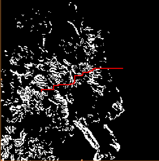
The Mathematica function FindShortestPath is now implemented to find the minimum distance path between the two user-entered coordinates::
path = Replace[FindShortestPath[pg, pix1, pix2], Except[_List] -> {}];
Now for a more in-depth analysis of the path finding mechanism...
Visualization of FindShortestPath
The connected "pixel plane" looks like this:
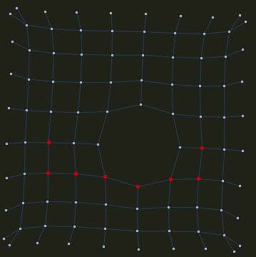
If a pixel is deleted using VertexDelete,
g = VertexDelete[graph, {Pixel[5, 5]}]
the resulting pixel plane looks like this:
When FindShortestPath is applied to two randomly chosen pixels on the plane,
FindShortestPath[g, Pixel[5, 3], Pixel[5, 8]]
the red dots show the shortest path.
However, if there is no path, an error message is produced:
    If[path === {},
    bin = bin;
    "Error: There is no path.",
Otherwise, a function "dropOne" is implemented in order to minimize the length of the path even further: dropOne drops points on the path (excluding starting and ending points) that will still give a path disjoint from the white pixels that have been deleted.
    bin = ImageMultiply[bin,
    Erosion[ReplacePixelValue[ConstantImage[White, $size],
    List @@@ path -> Black], 1]];
    fullTerrain = ImageAdjust@Image[QuantityMagnitude[data]];
    mag = ImageDimensions[fullTerrain]/$size;
    mesh = ImageMesh[bin, Method -> "Exact",
    DataRange -> Transpose[{{1, 1}, ImageDimensions[bin]}]];
    newPath = List @@@ path[[2 ;; -2]];
Definition:
    dropOne =
    Function[path,
    Replace[
    SelectFirst[Range[2, Length[path] - 1],
    RegionDisjoint[mesh, Line[Delete[path, #]]] &],
    {d_Integer :> Delete[path, d], _ :> path}
    ]];
The new, improved path, achieved using the dropOne function, is named "testPath":
testPath = FixedPoint[dropOne, newPath];
Notice how testPath improves the distance by "smoothening out" the path.
The scaled length of the path (aka the path length in pixels) is now determined by using the EuclideanDistance. The scaled distance is converted to actual distance in miles by using the "realPixelSize" value computed at the beginning using the pixelSize function:
    scaledLength =
    N@Total[EuclideanDistance @@@
    Partition[testPath, 2, 1]] (*with dropOne function*);
    actualLength = scaledLength*realPixelSize (*in miles*);
In this example with Denver and Aspen, the length of the path before dropOne was implemented was 128 miles while the length of the path after dropOne was implemented was 117.2 miles.
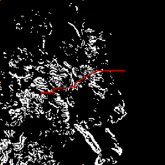
A grid is created to output a list of lists, specifically, a list of images: the raw graph representing the original path, the smoothened graph representing the improved graph after the dropOne function is implemented, the gradient graph showing the shortest path, and the full terrain image with relative elevations.
    Grid[{
    {"Raw Graph: ",
    ImageResize[HighlightImage[bin, Line[List @@@ path]], 500]},
    {"Smoothened Graph: ",
    ImageResize[HighlightImage[bin, Line[testPath]], 500]},
    {"Gradient: ",
    ImageResize[
    HighlightImage[
    ImageAdjust@
    GradientFilter[terrainImage,
    1], {Line[{##} - 0.5 & @@@ testPath]}], 500]},
    {"Terrain with path marked in red: ",
    HighlightImage[fullTerrain, {Line[mag*{##} & @@@ testPath]}]},
    {"Distance: ", actualLength}}], Alignment -> Left
    ]]
Further Work
A possible improvement that may be made is a quicker runtime: in fact, the image quality may be adjusted in my microsite in order to account for slow runtime. On the microsite, another problem is the need for the user to adjust the threshold in order to obtain the best possible graph: there should be a set numerical correlation between the actual gradient values and threshold since threshold is just a relative measurement of slope.


