Axon, also known as the nerve fiber, is a long, slender projection of a nerve cell, or neuron, that conducts electrical impulses known as action potentials, away from the nerve cell body. Although the connectivity of axons are crucial in signal transfer between neurons, its structural assembly and trend across the cortex is yet not widely investigated. By utilizing image processing techniques, we look at the structural trend and are able to quantify axon expressions, providing valuable data for further investigation of neuronal activity.

Background: What are Axons?

The neocortex, also called the neopallium and isocortex, is the part of the mammalian brain involved in higher-order brain functions such as sensory perception, cognition, generation of motor commands, spatial reasoning and language. The neocortex is the largest part of the cerebral cortex - outer layer of the cerebrum - in human brain.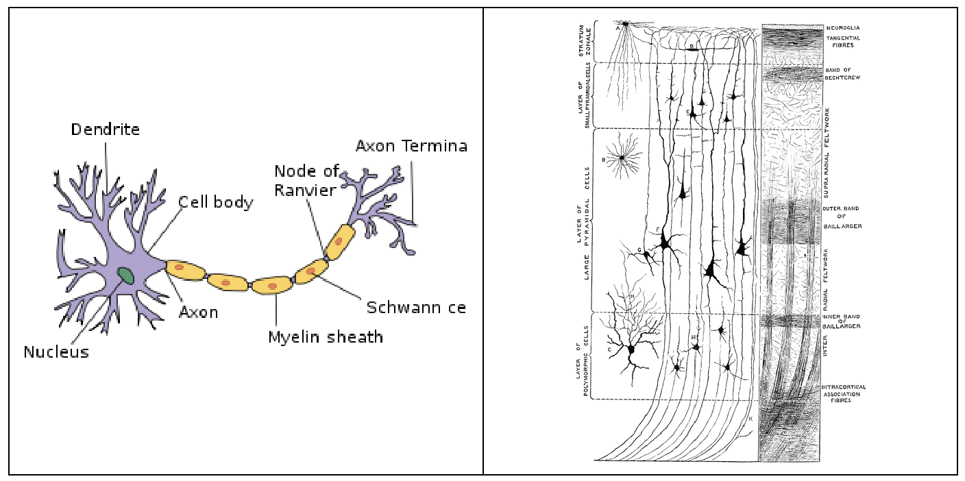

The neocortex is made up of six layers, labelled from the outermost inwards, I to VI. Since different layers specialize in different activities, analysis of changing trend in axon density across the layers is crucial to understanding brain activity. Plasticity over longer distances means that a larger number of neural circuits can be achieved and implies a larger memory capacity per synapse (Fawcett and Geller, 1998, Chen et al., 2002, Papadopoulos, 2002).

Axons span many millimeters of cortical territory, and individual axons target diverse areas (Zhang and Deschenes, 1998). Thus, understanding the repertoire of axonal structural changes is fundamental to evaluating mechanisms of functional rewiring in the brain.

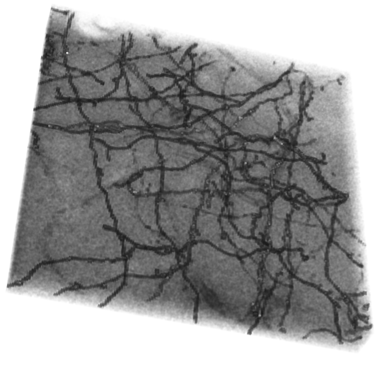
Images acquired from distinct axon arbors in adult barrel cortex of GFP transgenic mice were used in this project. Two-photon microscopy techniques were used along with SBEM(Serial Block-face scanning Electron Microscopy) techniques. Images were obtained after a series of surface scanning throughout the entire sample, then stacked for segmentation and quantification. Due to the size of the data, only the first section of layer 1 was analyzed in this project.

Import Images

In order to carry out an image analysis with electron-microscope images, image data (real-value pixel sizes corresponding to each pixels) is needed.

First we want to assign pixel sizes corresponding to real image sizes:

xpixelsize = 512Quantity[1,"Micrometers"];
ypixelsize = 512 Quantity[1,"Micrometers"];
zstepsize = 293Quantity[1,"Micrometers"];

Then we import the TIF dataset from directory.

pic=Import@URLDownload["https://github.com/JihyeonJe/JJ-WSS18/raw/master/axon.tif"];

Image Processing

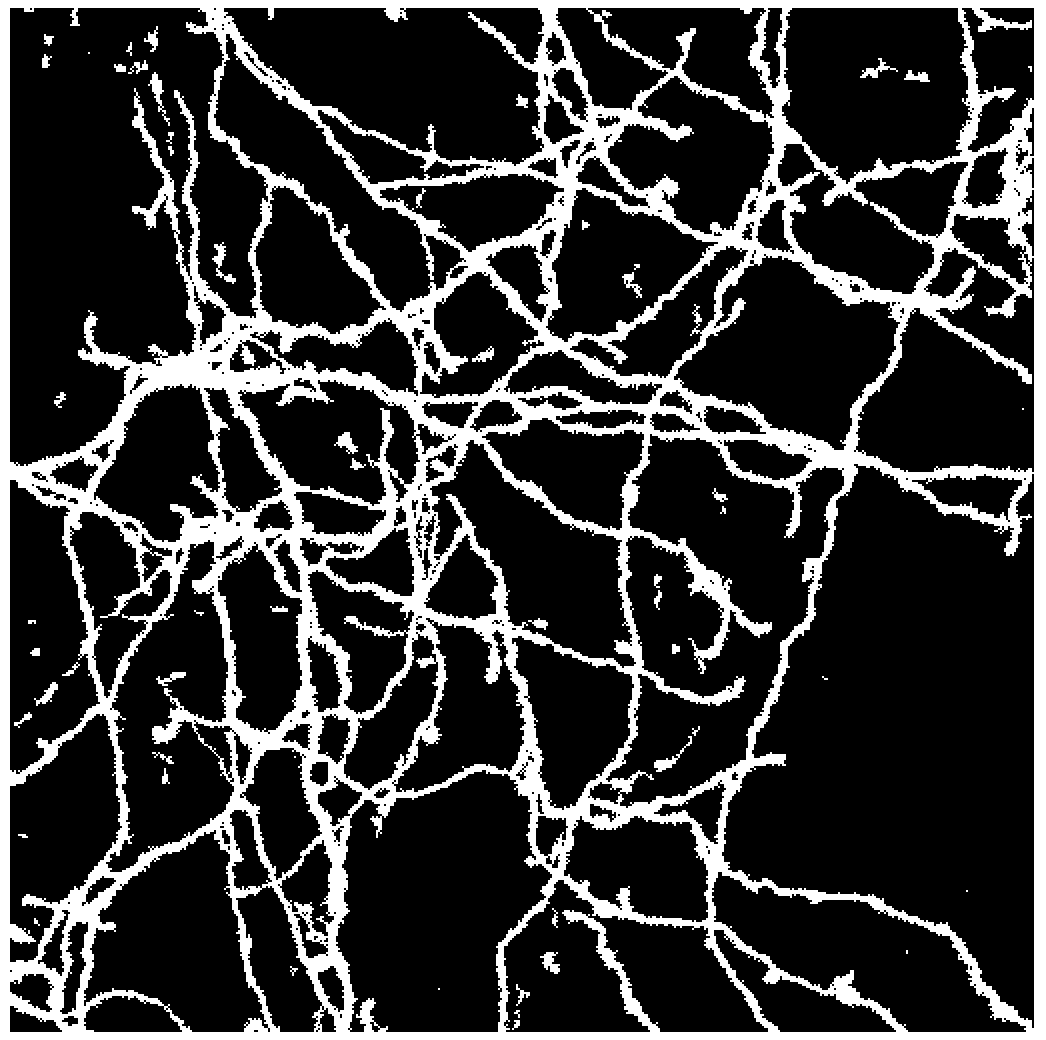
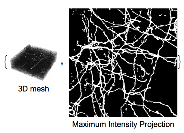
After images are imported, 3D mesh is created for visualization of general structural trend throughout the entire stack. Maximum intensity projection is also generated from the stacks to aid the understanding of overall axon distribution. To carry out density and volume calculations, images were binarized with given thresholds.

To get a general idea of the structure, we create a 3D mesh with the dataset:

image3D=Image3D[image,ColorFunction->"GrayLevelOpacity",BoxRatios->{1,1,1/3}];
resize = ImageResize[image3D, 170]

Then we binarize all the images with a set threshold:

binarized = Map[MorphologicalBinarize[#, {0.10, 0.4}]&,ImageAdjust/@image];

Now let's create maximum intensity projection from the previously created binarized images:

MIP = Image3DProjection[Image3D[binarized]]

Display mesh and temporal interpolation side by side for convenient analysis:

{Labeled[image3D,Text@"3D mesh"],Labeled[MIP,Text@"Maximum Intensity Projection"]}

Calculate volume and density

With processed images, we are now able to calculate volume and density of the axons expressed in the images. This step is crucial in analyzing the volumetric intensity of axon expression in the sample. Volume of total axons expressed were calculated by counting all non-zero elements in the binarized images and multiplying them by pixel sizes.

expressedvol = Count[Flatten[ImageData /@ binarized],1]*xpixelsize*ypixelsize*zstepsize

Then we get the value of 12353445560320 um^3.

Now calculate the volume of the entire image stack by counting image dimensions and multiplying it with pixel sizes:

totalvol = First[ImageDimensions[First[image]]]*xpixelsize*Last[ImageDimensions[First[image]]]*ypixelsize*Length[image]*zstepsize

This results in another volumetric quantity of 1208088401018880 um^3.

Using these two values, calculate the average axon volume:

denstiy = N[expressedvol/totalvol]Quantity[1,"Micrometers"]

Then we can get the output of average axon volume, 0.0102256 um^3.

By casting a sliding window across the entire image stack from top to bottom, the general trend of axon density was observed. Since connectivity between axons is a crucial in understanding brain activity, sliding window allows an analysis of the amount of shared data between axons across the brain.

slidingwindow[x_] := Count[Flatten[ImageData[x]],1]
SetAttributes[slidingwindow,Listable];
window = Total /@ MovingMap[slidingwindow, binarized, 2];

Now plot the graph:

Show[ListPlot[window/(First[ImageDimensions[First[image]]]* Last[ImageDimensions[First[image]]]*3), Joined -> True, PlotStyle->Thick, PlotLabel-> "Axon Density Across Z",LabelStyle->Directive[Bold],  AxesLabel->"Axon Density (\!\(\*TemplateBox[{InterpretationBox[\"\[InvisibleSpace]\", 1],RowBox[{SuperscriptBox[\"\\\"\[Micro]m\\\"\", \"3\"]}],\"micrometers cubed\",SuperscriptBox[\"\\\"Micrometers\\\"\", \"3\"]},\n\"Quantity\"]\))" ]]

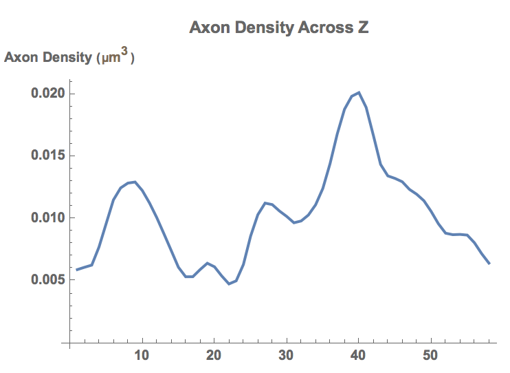
From the plotted graph we can see the general trend of axon density across the brain. For example, a local maxima(peak) at the region corresponding to the line of Gennari would indicate that the specific area is responsible for active neuronal signal transfer. When analyzed across the entire brain, such data can provide a novel understanding of axon expression and structures.

References

Image data acquired from Diadem Challenge - Neocortical Layer Axon 1 : http://www.diademchallenge.org/neocortical_layer_ 1axons readme.html

De Paola V1 et al. (2006) Cell type-specific structural plasticity of axonal branches and boutons in the adult neocortex. Cold Spring Harbor Symp. Quant. Neruon. 49, 861-875. DOI: 10.1016/j.neuron.2006.02.017

Author Information: Jihyeon Je (Western Reserve Academy, jej19@wra.net)