Introduction
We discuss the mechanics of yield curve bootstrapping and demonstrate how the use of linear solver speeds up the process. Once the market data for curve construction is available, the bootstrapping process is quite quick and the entire yield curve is obtained in a single step. This optimises the bootstrapping procedures and leads to an elegant and transparent solution. The auxiliary output - the so-called yield curve derivatives such as zero and forward rates can be generated on the fly.
The yield curve methodology
Yield curves are one of the most fundamental concepts in finance. Curves are basic building blocks for many financial instruments and they are key determinants of value creation due to the discounting effect. Yield curves - when built with derivative instruments - are essential for forward rates calculation. As such, they are critical component of the entire market for interest rate derivatives.
Yield curves are created through bootstrapping - a technique that converts market observable rates into 'zero-coupon' instruments. To be consistent and correct, the yield curve has to satisfy the following condition:
Sum[ c[[i]] g[[i]] DF[[i], {i,1, n-1}] + (1+c[[n]] g[[n]]) DF[[n]] ==1
where c is the fixed market rate, g is the year-fraction and DF stands for discount factor that we are trying to bootstrap
When we choose the 'fixed leg' method, the above expression guarantees that all instruments on the yield curve will price to par. This ensures that discount factors are correctly calculated.
The curve equation expression above ensures the consistency for a single curve pillar - i.e. the maturity point on the curve When $m$ such instruments are lined up together, we obtain a matrix of curve equations that we can solve with linear solver:
Curve bootstrapping - example
We demonstrate the curve building principles with the following simple example:
- Randomize market data for the curve construction
Visualise the data as the curve input
dim=30;
t=Table[0.5,{dim}];
act=Accumulate[t];
r=Table[1,{dim}];
c=0.0055+RandomReal[{0.005,0.009}] Sqrt[act];
td=TemporalData[c,{act}];
ListLinePlot[td,PlotStyle->{Blue, Thickness[0.008]},GridLines->{Automatic,Automatic},PlotLabel->Style["Yield curve market quotes",Purple,15]]
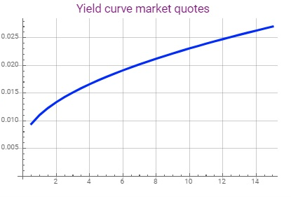
Using the market data above, we construct matrix of cash flows and use LinearSolve method to obtain the required discount factors.
z=Table[If[i<j,c[[i]]*t[[i]],If[i==j,r[[i]]+c[[i]]*t[[i]],0]],{j,1,dim},{i,1,dim}];
df=LinearSolve[z,r];
td2=TemporalData[df,{act}];
ListLinePlot[td2,PlotLabel->Style["Discount factors",Blue,15],GridLines->{Automatic, Automatic},PlotStyle->{Red,Thickness[0.009]}]
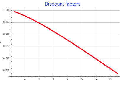
The obtained discount factors are unique, monotonically decreasing and in right order. Having discount factors computed allows us to obtain all kind of measures that depend on discount factors:
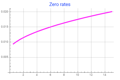
Zero-coupon rates These are the unique rates that pay out single cash flow at maturity and are essentially 'inverted' DF $zero rate = Log[1/DF]/T$
zc=Log[1/df]/act;
td3=TemporalData[zc,{act}];
ListLinePlot[td3,PlotLabel->Style["Zero rates",Blue,15],GridLines->{Automatic, Automatic},PlotStyle->{Magenta,Thickness[0.009]}]
Forward rates Forward rates are 'special' as they are rates observed today but starting in the future. They are market expectations of future short-term rates and therefore important indicators of future level of interest rates in the economy. We calculate a series of 3-monthly forward rates from the discount factors as follows:
forward_rate[t1,t2] =( DF[t1]/DF[t2]-1)/g[t1,t2]
where $t1$ and $t2$ are times in the future, $DF$ are discount factors at time point $t1$ and $t2$ and $g[t1,t2]$ is the year fraction between
time point $t1$ and $t2$, with $t2 >t1$
In order to compute forward rates, we need to introduce a simple function that computes the business day. That can be easily done using the built-in functional components:
OpenDay[start_,incr_,itype_]:=NestWhile[DatePlus[#,1]&,DatePlus[start,{incr,itype} ],Not[BusinessDayQ[#]]&]
and we can test it
OpenDay[Today,3,"Day"]
and get the correct day - Monday, 23rd July 18
To compute forward rates, we first generate forward dates, calculate the time interval, interpolate DF from the DF object and then use the forward rate formula to get the rate:
intdf=Interpolation[td2,Method->"Spline"];
fwdates=Table[OpenDay[Today,i,"Month"],{i,3,60,3}];
dd=DateDifference[%,"Year",DayCountConvention->"Actual360"];
Differences[dd];
kd=Mean[%][[1]];
fwrates=Table[(intdf[i]/intdf[i+kd]-1)/kd,{i,kd,60 kd, kd}]//Quiet;
td4=TemporalData[fwrates,{Range[kd,60 kd, kd]}];
ListLinePlot[td4,PlotTheme->"Web",PlotLabel->Style["Smooth Forward rates",Blue,15]]
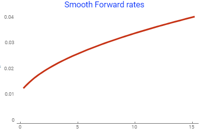
We have obtained smooth forward rates from the generated discount factors - this is an evidence that the discount factors were properly calculated and the choice of interpolation was appropriate.
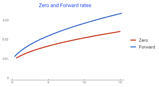
When the yield curve is upward sloping, then the mathematics of forward rates will cause forward rates being higher than the zero rates. We can see this is the case:
ListLinePlot[{td3,td4},PlotTheme->"Web",PlotLabel->Style["Zero and Forward rates",Blue,15], PlotLegends->{"Zero", "Forward"}]
Real-case example
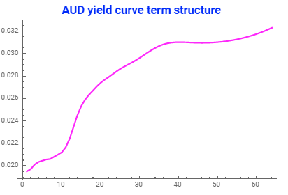
Having explained the yield curve bootstrapping methodology, we can now move to the real-case scenario where we will the actual market data to construct the Australian Dollar (AUD) curve. We use deposit rates in the short-end and the swap rates in the mid-to-long end of the curve with maturity up to 30 years. The swap will pay out semi-annually.
pmfreq=2;
pildates={OpenDay[Today,1, "Month"],OpenDay[Today,2, "Month"],  Table[OpenDay[Today, 3 i, "Month"],{i,4}],OpenDay[Today,18, "Month"], Table[OpenDay[Today, i, "Year"],{i,2,10 }], OpenDay[Today,12, "Year"],OpenDay[Today,15, "Year"],OpenDay[Today,20, "Year"],OpenDay[Today,25, "Year"],OpenDay[Today,30, "Year"]}//Flatten;
pilyrs=DateDifference[pildates   ,"Year",DayCountConvention->"Actual365"][[All,1]] ;
crvQ={0.0195,0.0197,0.0201,0.02034,0.02045,0.02056,0.0206,0.0208,0.0212,0.0224,0.0245,0.0259,0.0267,0.0274,0.0279,0.0284,0.0292,0.0305,0.03097,0.0312,0.0323};
tdQ=TemporalData[crvQ,{pilyrs}];
intQ=Interpolation[tdQ ,Method->"Spline"];
crvD=Length[crvQ];
cfdates={Today,OpenDay[Today,1, "Month"],OpenDay[Today,2, "Month"],  Table[OpenDay[Today, 3 i, "Month"],{i,4}],Table[OpenDay[Today, (12/pmfreq ) i, "Month"],{i,3,30 pmfreq }]}//Flatten;
cfyrs=Drop[DateDifference[cfdates   ,"Year",DayCountConvention->"Actual365"][[All,1]],1];
cfyD=Length[cfyrs ];
intrates=intQ [cfyrs ];
ListLinePlot[intrates,PlotLabel->Style["AUD yield curve term structure",Blue,{15,Bold}],PlotStyle->{Magenta, Thick}]
We first split the market data into (i) deposits and (ii) swap segments:
depoyrs={Take[ cfyrs ,3],Differences[Take[cfyrs,{3,6}]]}//Flatten;
fraAv=Take[depoyrs,-4]//Mean;
swapData=Inner[{#1,#2}&,Drop[cfyrs,6] ,Drop[intrates ,6],List];
swapyrs={0,cfyrs[[4]],cfyrs[[6]] ,Take[cfyrs,{7,cfyD}]}//Flatten;
swyfrac=Differences[swapyrs ];
swyAv=Mean[swyfrac];
swapD=Length[swapData];
and built the matrix of linear equations that we solve for the discount factors:
zTab1=Table[If[i==j,1+intrates[[j]] If[i<=2,depoyrs [[i]],fraAv ],0],{j,6},{i,cfyD}];
zTab2=Table[If[MemberQ[swapyrs,cfyrs[[i]]],If[cfyrs[[i]]<swapData[[j,1]],swapData[[j,2]] swyAv ,If[cfyrs[[i]]==swapData[[j,1]],1+swapData[[j,2]] swyAv  ,0]],0],{j,swapD},{i,1,cfyD}];
zTab0=Join[zTab1,zTab2];
b1Vec=ConstantArray[1,cfyD];
dfact=LinearSolve[zTab0 ,b1Vec ];
tdDf=TemporalData[dfact,{cfyrs}]//Quiet;
ListLinePlot[tdDf   ,PlotLabel->Style["Generated Discount factors",Blue,15],PlotStyle->{Thickness[0.01],Purple},PlotRange->{Full,{1,0.3}},InterpolationOrder->2]
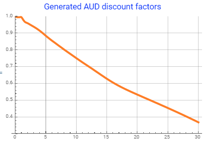
This is the actual AUD yield curve built from derivative instruments that can be used to value various AUD instruments.
Curve smoothing
Since we use the actual market data, the generated discount factors are not as smooth as in our first example. This is particularly visible in the short-end of the curve. The existence of kinks is due to several factors - different segments of the the curve are being traded by different desks and equilibrium market rates are obtained through different price discovery. If curve kinks and peaks are undesirable, there exist several techniques to smooth them sway and we look at linear filters that can help to accomplish this task. The built-in Mathematica GaussianFilter is particularly useful as it provides required level of control to manipulate 'noisy' data.
For example, applying GaussianFilter with radius $r$ = 3 and standard deviation $sigma$ =2 provide nice and smooth output the the 'kinky' segment of the curve:
iDF=Interpolation[tdDf,Method->"Spline"];
tdDF2=TemporalData[Map[iDF,Range[0.25,30,0.25]] ,{Range[0.25,30,0.25]}];
orD=iDF/@Range[0.25,30,0.25];
flD=GaussianFilter[orD,{3,2}];
ListLinePlot[{Take[orD ,10],Take[flD,10]},PlotLabel->Style["Curve correction with Gaussian filter",Blue,15],PlotLegends->{"Original", "Filtered"},PlotStyle->{Thickness[0.008],Thickness[0.008]},InterpolationOrder->3]
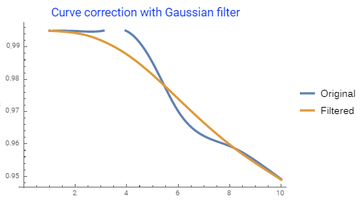
The filtered output produces decent curve with smoother short-end that, if needed, can be used to construct all types of derivatives with appropriate rates. It has to be noted that the filter can be applied both to (i) discount factors and/or (ii) forward rates - depending on the required objective. Generally, the higher the radius, the smoother the output.
Conclusion
The usage of linear solver and its application in curve bootstrapping leads to fast and accurate curve construction with unique discount factors. The function can be easily applied to any environment where the term structure of market data is duly defined. We have also demonstrated the use of filtering technique for curve smoothing with built-in Mathematica filters that provide rexcellent tool for output manipulation if the curve kinks become an issue.