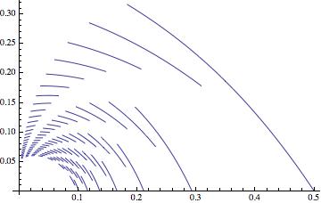
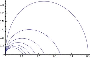
Thank you Vitaliy for rising up this question. The following snippets of Mathematica code show how one can derive the analytical curves that connect the critical points. Let's start with eq (1):
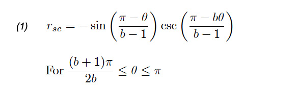
Show[Table[
PolarPlot[
Sin[(\[Pi] - \[Theta])/(b - 1)] Csc[(b (\[Pi] - \[Theta]))/(
b - 1)], {\[Theta], (b + 1) \[Pi]/(2 b), \[Pi]}], {b, 2, 30, 1}],
PlotRange -> All]
We take the values of theta in the critical points and then we express b as function of theta:
Solve[(b + 1) \[Pi]/(2 b) == \[Theta], b]
Then we replace b in eq (1)
Sin[(\[Pi] - \[Theta])/(b - 1)] Csc[(b (\[Pi] - \[Theta]))/(
b - 1)] /. {b -> -(\[Pi]/(\[Pi] - 2 \[Theta]))} // FullSimplify
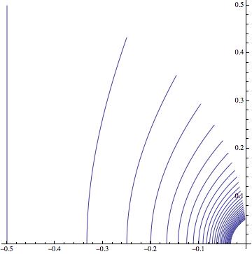
This gives us r = -Cos(Theta) which links together the critical points:
Show[PolarPlot[-Cos[\[Theta]], {\[Theta], \[Pi]/2, \[Pi]}],
Table[PolarPlot[
Sin[(\[Pi] - \[Theta])/(b - 1)] Csc[(b (\[Pi] - \[Theta]))/(
b - 1)], {\[Theta], (b + 1) \[Pi]/(2 b), \[Pi]},
PlotStyle -> {Red}], {b, 2, 30, 1}], PlotRange -> All]
To find the rest of critical lines for Down Self-Contacting n-ary trees we can use either eq (2) or eq (3).
(3)
Show[Table[
Table[PolarPlot[(
Sin[(\[Pi] (3 - 2 n) - \[Theta] (b - 2 n + 2))/(b - 1)] +
Sqrt[-(4 Cos[(2 (\[Pi] - \[Theta]))/(b - 1)]) +
4 Cos[(2 (\[Pi] - \[Theta]) (n - 2))/(b - 1)] -
4 Cos[(2 (\[Pi] - \[Theta]) (n - 1))/(b - 1)] -
Cos[(2 \[Theta] (b - 2 n + 2) + \[Pi] (4 n - 6))/(b - 1)] + 5]/
Sqrt[2])/(
2 (Sin[(\[Pi] - \[Theta])/(b - 1)] +
Sin[((\[Pi] - \[Theta]) (2 n - 3))/(b - 1)])), {\[Theta], ((5 +
b - 4 n) \[Pi])/(2 (2 + b - 2 n)), ((7 + b - 4 n) \[Pi])/(
2 (3 + b - 2 n))}], {b, 4 n - 5, 30, 1}], {n, 2, 8, 1}],
PlotRange -> All]
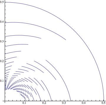
(2)
Show[Table[
Table[PolarPlot[(
Sin[(\[Pi] (3 - 2 n) - \[Theta] (b - 2 n + 2))/(b - 1)] +
Sqrt[-(4 Cos[(2 (\[Pi] - \[Theta]))/(b - 1)]) -
Cos[(2 \[Theta] (b - 2 n + 2) + \[Pi] (4 n - 6))/(b - 1)] +
4 Cos[(2 (\[Theta] (b - n + 1) + \[Pi] (n - 2)))/(b - 1)] -
4 Cos[(2 (-(b \[Theta]) + \[Theta] n - \[Pi] n + \[Pi]))/(
b - 1)] + 5]/Sqrt[2])/(
2 (Sin[(\[Pi] - \[Theta])/(b - 1)] +
Sin[(2 b \[Theta] + \[Theta] - 2 \[Theta] n + 2 \[Pi] n -
3 \[Pi])/(b - 1)])), {\[Theta], ((3 + b - 4 n) \[Pi])/(
2 (1 + b - 2 n)), ((5 + b - 4 n) \[Pi])/(2 (2 + b - 2 n))}], {b,
4 n - 3, 30, 1}], {n, 2, 8, 1}], PlotRange -> All]
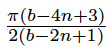
In eq (2) we can take two types of critical angles,
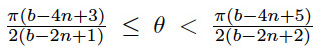
. We take the first type.
Solve[\[Theta] == ((3 + b - 4 n) \[Pi])/(2 (1 + b - 2 n)), b]
Then we replace this expression of b in (2)
(Sin[(\[Pi] (3 - 2 n) - \[Theta] (b - 2 n + 2))/(b - 1)] +
Sqrt[-(4 Cos[(2 (\[Pi] - \[Theta]))/(b - 1)]) -
Cos[(2 \[Theta] (b - 2 n + 2) + \[Pi] (4 n - 6))/(b - 1)] +
4 Cos[(2 (\[Theta] (b - n + 1) + \[Pi] (n - 2)))/(b - 1)] -
4 Cos[(2 (-(b \[Theta]) + \[Theta] n - \[Pi] n + \[Pi]))/(
b - 1)] + 5]/Sqrt[2])/(
2 (Sin[(\[Pi] - \[Theta])/(b - 1)] +
Sin[(2 b \[Theta] + \[Theta] - 2 \[Theta] n + 2 \[Pi] n -
3 \[Pi])/(b - 1)])) /. {b -> (-3 \[Pi] + 4 n \[Pi] +
2 \[Theta] - 4 n \[Theta])/(\[Pi] - 2 \[Theta])} // FullSimplify
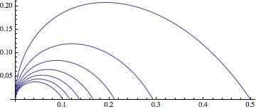
obtaining thus the desired critical equations for the angles
.
Show[Table[
PolarPlot[(
2 Cos[(5 \[Pi] - 4 n \[Pi] - 2 \[Theta])/(4 - 4 n)] + Sqrt[
10 - 6 Cos[(\[Pi] - 2 \[Theta])/(2 - 2 n)] + 8 Sin[\[Theta]] -
8 Sin[(\[Pi] - 2 n \[Theta])/(2 - 2 n)]])/(
4 (Cos[(\[Pi] + 2 \[Theta] - 4 n \[Theta])/(4 - 4 n)] +
Sin[(\[Pi] - 2 \[Theta])/(4 (-1 + n))])), {\[Theta], 0,
Pi/2}], {n, 2, 8, 1}], PlotRange -> All]
For the angles
a similar expression can be found:
Solve[\[Theta] == ((5 + b - 4 n) \[Pi])/(2 (2 + b - 2 n)), b]
We replace b in eq (2)
(Sin[(\[Pi] (3 - 2 n) - \[Theta] (b - 2 n + 2))/(b - 1)] +
Sqrt[-(4 Cos[(2 (\[Pi] - \[Theta]))/(b - 1)]) -
Cos[(2 \[Theta] (b - 2 n + 2) + \[Pi] (4 n - 6))/(b - 1)] +
4 Cos[(2 (\[Theta] (b - n + 1) + \[Pi] (n - 2)))/(b - 1)] -
4 Cos[(2 (-(b \[Theta]) + \[Theta] n - \[Pi] n + \[Pi]))/(
b - 1)] + 5]/Sqrt[2])/(
2 (Sin[(\[Pi] - \[Theta])/(b - 1)] +
Sin[(2 b \[Theta] + \[Theta] - 2 \[Theta] n + 2 \[Pi] n -
3 \[Pi])/(b - 1)])) /. {b -> (-5 \[Pi] + 4 n \[Pi] +
4 \[Theta] - 4 n \[Theta])/(\[Pi] - 2 \[Theta])} // FullSimplify
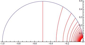
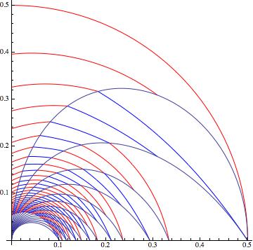
Finally we can merge these critical lines with eq (2) and (3).
Show[Table[
Table[PolarPlot[(
Sin[(\[Pi] (3 - 2 n) - \[Theta] (b - 2 n + 2))/(b - 1)] +
Sqrt[-(4 Cos[(2 (\[Pi] - \[Theta]))/(b - 1)]) -
Cos[(2 \[Theta] (b - 2 n + 2) + \[Pi] (4 n - 6))/(b - 1)] +
4 Cos[(2 (\[Theta] (b - n + 1) + \[Pi] (n - 2)))/(b - 1)] -
4 Cos[(2 (-(b \[Theta]) + \[Theta] n - \[Pi] n + \[Pi]))/(
b - 1)] + 5]/Sqrt[2])/(
2 (Sin[(\[Pi] - \[Theta])/(b - 1)] +
Sin[(2 b \[Theta] + \[Theta] - 2 \[Theta] n + 2 \[Pi] n -
3 \[Pi])/(b - 1)])), {\[Theta], ((3 + b - 4 n) \[Pi])/(
2 (1 + b - 2 n)), ((5 + b - 4 n) \[Pi])/(2 (2 + b - 2 n))},
PlotStyle -> {Blue}], {b, 4 n - 3, 30, 1}], {n, 2, 8, 1}],
Table[Table[
PolarPlot[(
Sin[(\[Pi] (3 - 2 n) - \[Theta] (b - 2 n + 2))/(b - 1)] +
Sqrt[-(4 Cos[(2 (\[Pi] - \[Theta]))/(b - 1)]) +
4 Cos[(2 (\[Pi] - \[Theta]) (n - 2))/(b - 1)] -
4 Cos[(2 (\[Pi] - \[Theta]) (n - 1))/(b - 1)] -
Cos[(2 \[Theta] (b - 2 n + 2) + \[Pi] (4 n - 6))/(b - 1)] + 5]/
Sqrt[2])/(
2 (Sin[(\[Pi] - \[Theta])/(b - 1)] +
Sin[((\[Pi] - \[Theta]) (2 n - 3))/(b - 1)])), {\[Theta], ((5 +
b - 4 n) \[Pi])/(2 (2 + b - 2 n)), ((7 + b - 4 n) \[Pi])/(
2 (3 + b - 2 n))}, PlotStyle -> {Red}], {b, 4 n - 5, 30, 1}], {n,
2, 8, 1}],
Table[PolarPlot[(
2 Cos[(5 \[Pi] - 4 n \[Pi] - 2 \[Theta])/(4 - 4 n)] + Sqrt[
10 - 6 Cos[(\[Pi] - 2 \[Theta])/(2 - 2 n)] + 8 Sin[\[Theta]] -
8 Sin[(\[Pi] - 2 n \[Theta])/(2 - 2 n)]])/(
4 (Cos[(\[Pi] + 2 \[Theta] - 4 n \[Theta])/(4 - 4 n)] +
Sin[(\[Pi] - 2 \[Theta])/(4 (-1 + n))])), {\[Theta], 0,
Pi/2}], {n, 2, 8, 1}],
Table[PolarPlot[(-1 + Sqrt[
3 - 2 Cos[(\[Pi] - 2 \[Theta])/(3 - 2 n)] -
2 Sin[(\[Pi] + 4 (-2 + n) \[Theta])/(6 - 4 n)] +
2 Sin[(\[Pi] + 4 \[Theta] - 4 n \[Theta])/(-6 + 4 n)]])/(
2 (Cos[\[Theta]] +
Sin[(\[Pi] - 2 \[Theta])/(-6 + 4 n)])), {\[Theta], 0,
Pi/2}], {n, 2, 8, 1}], PlotRange -> All]
The same procedure can be extended to the Up symmetric trees equations.


