Message Boards Message Boards

6
|
18831 Views
|
20 Replies
|
39 Total Likes
View groups...
Share
Share this post:

Closed spline going through points

Posted 11 years ago
In the BSplineCurve documentation, under applications / interpolation, instructions for making an open curve going through points is given. 

Similar code is in the Demonstration Knot Vector Generation for B-Spline Interpolation.  It also does open curves. 

I'd like something similar for closed curves.  Given 16 or so points, generate a smooth closed curve going through those points.  

I'm hoping to make a new Demonstration on the Inscribed square problem. The conjecture is that every closed curve has an embedded square.  My idea is to randomly generate the points of 4 squares, do a Traveling Salesman on those points, then draw the interpolated spline through the 16 points.

POSTED BY: Ed Pegg
20 Replies
And here the reverse problem:
 CreateScene[pts_List,{a_,b_}]:=Module[{points,order,smooth,splinepoints,splnfunc,p1,p2,p3,p4,d,e},
 order=FindShortestTour[pts][[2]];
 points=pts[[order]];
 splinepoints={#2,#2+Normalize[#3-#] Norm[#3-#2]/3,#3-Normalize[#4-#2] Norm[#3-#2]/3,#3}&@@@Partition[points,4,1,{2,2}];
 smooth=BSplineCurve[Flatten[splinepoints,1],SplineDegree->3];
 splnfunc=BSplineFunction[Flatten[splinepoints,1],SplineDegree->3];
 p1=splnfunc[a];
 p2=splnfunc[b];
 d=p2-p1;
e={-1,1}Reverse[d];
p3=e+p2;
p4=p3-d;
Graphics[{smooth,Blue,PointSize[0.04],Point[p1],Black,Point[p2],Green,Point[p3],Point[p4]},PlotRange->3/2]
]
pt0=RandomReal[{-1,1},{6,2}];
Manipulate[CreateScene[pt,{a,b}],{{pt,pt0},Locator,Appearance->Graphics[{Red,PointSize[0.02],Point[{0,0}]}]},{{a,0},0,1},{{b,0.5},0,1}]
giving:

You can freely move the 6 red points, and move the blue and black dots around the contour, the greens one are created and should fit on the contour.
POSTED BY: Sander Huisman
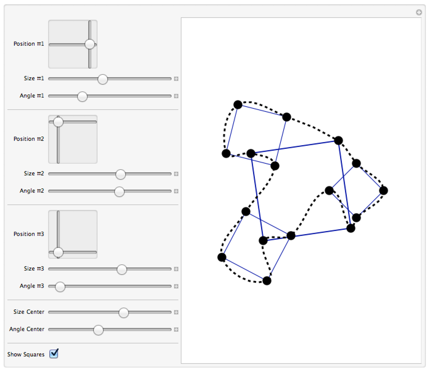
Here I made the interactive example:
 ClearAll[CreateSquare,CreateScene]
 CreateSquare[p:{px_,py_},L_,\[Theta]_]:=With[{\[Phi]=Range[0,3\[Pi]/2,\[Pi]/2]+\[Theta]}, {px+Cos[\[Phi]]L/2,py+Sin[\[Phi]]L/2}\[Transpose]]
 CreateScene[p:{p1_,p2_,p3_},L:{l1_,l2_,l3_,l4_},\[Theta]:{\[Theta]1_,\[Theta]2_,\[Theta]3_,\[Theta]4_},showsqrs_]:=Module[{plg,allpoints,order,smooth},
 plg=MapThread[CreateSquare,{Append[p,{0,0}],L,\[Theta]}];
 allpoints=Flatten[plg,1];
 order=FindShortestTour[allpoints][[2]];
 allpoints=Part[allpoints,order];
 smooth=BSplineCurve@{#2,#2+Normalize[#3-#] Norm[#3-#2]/3,#3-Normalize[#4-#2] Norm[#3-#2]/3,#3}&@@@Partition[allpoints,4,1,{2,2}];
 If[showsqrs,
Graphics[{EdgeForm[{Darker@Blue,Thickness[0.003]}],FaceForm[None],Polygon[Most@plg],{EdgeForm[Thickness[0.005]],Polygon[Last@plg]},Black,PointSize[0.04],Point[allpoints],CapForm[None],Dashing[0.0125],Thickness[0.008],smooth},PlotRange->2]
,
Graphics[{Black,CapForm[None],Dashing[0.0125],Thickness[0.008],smooth},PlotRange->2]
]
]
Manipulate[
CreateScene[{p1,p2,p3},{size1,size2,size3,size4},{\[Theta]1,\[Theta]2,\[Theta]3,\[Theta]4},show]
,
{{p1,{1,0},"Position #1"},{-1,-1},{1,1}},
{{size1,0.98,"Size #1"},0.2,2},
{{\[Theta]1,1.57,"Angle #1"},0,2\[Pi]},
Delimiter,
{{p2,{-0.8,1},"Position #2"},{-1,-1},{1,1}},
{{size2,1.28,"Size #2"},0.2,2},
{{\[Theta]2,3.68,"Angle #2"},0,2\[Pi]},
Delimiter,
{{p3,{-0.8,-1},"Position #3"},{-1,-1},{1,1}},
{{size3,1.3,"Size #3"},0.2,2},
{{\[Theta]3,0.3,"Angle #3"},0,2\[Pi]},
Delimiter,
{{size4,2.25,"Size Center"},1,3},
{{\[Theta]4,0.21,"Angle Center"},0,2\[Pi]},
Delimiter,
{{show,True,"Show Squares"},{True,False}}
]
giving:
POSTED BY: Sander Huisman
I had an error in my code, the L/2 was outside the braces, now it is inside. I updated the above post.
POSTED BY: Sander Huisman
Posted 11 years ago
These curves look gorgeous.  

I was thinking of combining the Demonstration A Polygon from Its Midpoints with Vitaly's midpoint-based code.  These curves that are generated look very nice -- I'd want to be able to switch the squares on and off -- is it possible to spot where a square might be in a curve?
POSTED BY: Ed Pegg
Posted 11 years ago
I've started the packages for "Square", "Spline interpolation", and the "Inscribed square problem" on Wikicode.

POSTED BY: Michael Hale
I think I kinda made what the author requested:
 ClearAll[CreateSquare,CreateRandomSquares,CreateScene]
 CreateSquare[p:{px_,py_},L_,\[Theta]_]:=Module[{\[Phi]},\[Phi]=Range[0,3\[Pi]/2,\[Pi]/2]+\[Theta]; {px+Cos[\[Phi]]L/2,py+Sin[\[Phi]]L/2}\[Transpose]]
 CreateRandomSquares[n_]:=Module[{r,L,\[Phi],\[Theta],sqrs},r=RandomReal[{0.2,0.45},n];
 \[Phi]=Range[0,(1-1/n)2\[Pi],2\[Pi]/n];
 \[Theta]=RandomReal[{0,2\[Pi]},n];
 L=RandomReal[{0.3,0.5},n];
 sqrs=MapThread[CreateSquare[#1{Cos[#3],Sin[#3]},#2,#4]&,{r,L,\[Phi],\[Theta]}];
 Append[sqrs,CreateSquare[{0,0},0.75,RandomReal[{0,2\[Pi]}]]]]
 CreateScene[]:=Module[{plg,allpoints,order,smooth},plg=CreateRandomSquares[3];
allpoints=Flatten[plg,1];
order=FindShortestTour[allpoints][[2]];
allpoints=Part[allpoints,order];
smooth=BSplineCurve@{#2,#2+Normalize[#3-#] Norm[#3-#2]/3,#3-Normalize[#4-#2] Norm[#3-#2]/3,#3}&@@@Partition[allpoints,4,1,{2,2}];
Graphics[{EdgeForm[{Darker@Blue,Thickness[0.003]}],FaceForm[None],Polygon[Most@plg],{EdgeForm[Thickness[0.005]],Polygon[Last@plg]},Black,PointSize[0.04],Point[allpoints],Dashing[0.025],Thickness[0.008],smooth}]]
pic=CreateScene[];
Button["Click Here",pic=CreateScene[]]
Dynamic[pic]
giving:
POSTED BY: Sander Huisman
This is really nice thinking Michael- great!
POSTED BY: Vitaliy Kaurov
Posted 11 years ago
@Sander, Thanks! It is probably better to scale the "handle lengths" based on the distance to the next point, so it looks smoother when the points are less evenly spaced.
Manipulate[
Graphics[BSplineCurve@{#2, #2 +
       Normalize[#3 - #] Norm[#3 - #2]/3, #3 -
       Normalize[#4 - #2] Norm[#3 - #2]/3, #3} & @@@
   Partition[pts, 4, 1, {2, 2}],
  ImageSize -> {400,
    300}], {{pts, {{0, 0}, {1, 0}, {2, .5}, {1, 1}, {0, 1}}}, Locator,
   LocatorAutoCreate -> True}]
POSTED BY: Michael Hale
@Michael

That is very very neat! wow! Nice way of using Partition to make it cyclic!
POSTED BY: Sander Huisman
Posted 11 years ago
Truthfully, based on my experience with Photoshop and other programs that let you draw splines I wouldn't have approached this in a manner as mathematically elegant as the example in the documentation. This is closer to Vitaliy's last post.
Manipulate[
Graphics[BSplineCurve@{#2, #2 + (#3 - #)/4, #3 - (#4 - #2)/4, #3} & @@@
    Partition[pts, 4, 1, {2, 2}],
  ImageSize -> {400,
    300}], {{pts, {{0, 0}, {1, 0}, {2, .5}, {1, 1}, {0, 1}}}, Locator,
   LocatorAutoCreate -> True}]
POSTED BY: Michael Hale
Posted 9 years ago
POSTED BY: Shutao Tang
Posted 9 years ago
POSTED BY: Michael Hale
Posted 9 years ago
POSTED BY: Shutao Tang
Posted 9 years ago
POSTED BY: Michael Hale
There is also another approach. For SplineDegree -> 2 the centers of segments connecting the points are always on the curve:
Manipulate[
Graphics[{BSplineCurve[pts, SplineClosed -> True, SplineDegree -> 2],
          {Red, PointSize[Large], Point[Mean /@ Partition[pts, 2, 1, 1]]}},
          ImageSize -> {400, 300}],
{{pts, {{0, 0}, {1, 0}, {2, .5}, {1, 1}, {0, 1}}}, Locator, LocatorAutoCreate -> True}]

POSTED BY: Vitaliy Kaurov
@Vitaliy @Michael

Indeed; if you look at the matrix m that is created you see that in certain rows only 1 non-zero value is. A neat way would be to make it a n-diagonal matrix with the two corners (top right, bottom left) filled with some numbers in order to make it cyclic.
POSTED BY: Sander Huisman
Posted 11 years ago
Maybe you would want to copy the first 4 points to the end of the list instead of just the first point. That would help with the continuity issue if you adjusted the basis matrix so that the first 4 elements in the first row were the same as the last 4 elements in the last row. I'd need to think about it some more.
POSTED BY: Michael Hale
This is neat idea to make the last point to be equal to the first to make a loop. And I think you are talking about this example. But I think the joining point behaves differently then the rest. It seems to me derivative is discontinues there. Here a quick manipulate to play with:
 Manipulate[
  pts = Append[pt, First[pt]];
  n = Length[pts];
  dist = Accumulate[
    Table[EuclideanDistance[pts[[i]], pts[[i + 1]]], {i,
      Length[pts] - 1}]];
  param = N[Prepend[dist/Last[dist], 0]];
  knots = Join[ConstantArray[0, 3], Range[0, 1, 1/(n - 3)],
    ConstantArray[1, 3]];
m = Table[
   BSplineBasis[{3, knots}, j - 1, param[[i]]], {i, n}, {j, n}];
ctrlpts = LinearSolve[m, pts];
ListPlot[pts, Prolog -> BSplineCurve[ctrlpts],
  PlotStyle -> Directive[Red, PointSize[Large]],
  PlotRangePadding -> 1/2, Frame -> True, Axes -> False]
, {{pt, {{1, 1}, {2, 1.25}, {2, 2}, {1.5, 2.75}, {1, 3}, {0.5,
     2.5}, {0.5, 1.1}}}, Locator, Appearance -> None,
  LocatorAutoCreate -> True}]

POSTED BY: Vitaliy Kaurov
I just played around with it but I'm not fully up-to-date how the knots are implemented and the syntax, but I generalized the example:
 pts={{1,1},{2,1.25},{2,2},{1.5,2.75},{1,3},{0.5,2.5},{0.5,1.1},{1,1}};
 n=Length[pts];
 dist=Accumulate[Table[EuclideanDistance[pts[[i]],pts[[i+1]]],{i,Length[pts]-1}]];
 param=N[Prepend[dist/Last[dist],0]];
 knots=Join[ConstantArray[0,3],Range[0,1,1/(n-3)],ConstantArray[1,3]];
 m=Table[BSplineBasis[{3,knots},j-1,param[[i]]],{i,n},{j,n}];
 MatrixForm[m]
 ctrlpts=LinearSolve[m,pts];
 ListPlot[pts,Prolog->{Blue,Arrow[pts],Black,BSplineCurve[ctrlpts]},PlotStyle->Directive[Red,PointSize[Large]],PlotRangePadding->1/2]

You can add points and so on, I think what has to be is, is the following: As you can see the matrix that is solved is quad-diagonal, I think we need some terms in the top-right and bottom-left of the matrix on order to make the spline 'cyclic'. I'm yet to figures out how to do that... but that is the idea I think...
POSTED BY: Sander Huisman
I think it is pretty neat idea for a Demonstration. Making a closed spline is pretty easy though. It is mentioned in the same documentation article a little deep down. Basically 
pts = RandomReal[1, {16, 2}];
Graphics[{BSplineCurve[pts, SplineClosed -> True], {Red, PointSize[Large], Point[pts]}}]


But according to that picture you are probably looking for curve passing through points - so you would need an interpolation. There is spline-based interpolation, but thankfully there is a simpler trick. If you repeat every point a few times - even only two - spline becomes very close to points. You can control how close with how many times you repeat same point and with option SplineDegree:
Graphics[{BSplineCurve[Flatten[Thread[{pts, pts}], 1],
   SplineClosed -> True, SplineDegree -> 3], {Red, PointSize[Large], Point[pts]}}]


BTW this cool Demonstration by Jaime Rangel-Mondragon uses closed spline:

The Path of the Rear Wheels of a Bus

POSTED BY: Vitaliy Kaurov
Reply to this discussion
Community posts can be styled and formatted using the Markdown syntax.
Reply Preview
Attachments
Remove
or Discard

Group Abstract Group Abstract