I will show the working code and the solution to task 2

t0 = 9; P = 14; lr = 1; g = 9.8; m = 1; ks = 100; kd = 10;
eqns = {Table[
    m*x[i]''[t] == -ks*(Sqrt[(x[i][t] - x[i - 1][t])^2 + (y[i][t] - 
              y[i - 1][t])^2] - lr)*(x[i][t] - x[i - 1][t])/
        Sqrt[(x[i][t] - x[i - 1][t])^2 + (y[i][t] - y[i - 1][t])^2] - 
      ks*(Sqrt[(x[i][t] - x[i + 1][t])^2 + (y[i][t] - 
              y[i + 1][t])^2] - lr)*(x[i][t] - x[i + 1][t])/
        Sqrt[(x[i][t] - x[i + 1][t])^2 + (y[i][t] - y[i + 1][t])^2] - 
      kd*(x[i]'[t] - x[i - 1]'[t]) - kd*(x[i]'[t] - x[i + 1]'[t]), {i,
      2, P - 1}], 
   Table[m*y[i]''[
       t] == -ks*(Sqrt[(x[i][t] - x[i - 1][t])^2 + (y[i][t] - 
              y[i - 1][t])^2] - lr)*(y[i][t] - y[i - 1][t])/
        Sqrt[(x[i][t] - x[i - 1][t])^2 + (y[i][t] - y[i - 1][t])^2] - 
      ks*(Sqrt[(x[i][t] - x[i + 1][t])^2 + (y[i][t] - 
              y[i + 1][t])^2] - lr)*(y[i][t] - y[i + 1][t])/
        Sqrt[(x[i][t] - x[i + 1][t])^2 + (y[i][t] - y[i + 1][t])^2] - 
      kd*(y[i]'[t] - y[i - 1]'[t]) - kd*(y[i]'[t] - y[i + 1]'[t]) - 
      m*g, {i, 2, P - 1}]};
ic = {Table[y[i]'[0] == 0, {i, 1, P}], Table[y[i][0] == 0, {i, 1, P}],
    Table[x[i][0] == lr*(i - 1), {i, 1, P}], 
   Table[x[i]'[0] == 0, {i, 1, P}]};
bc = {x[P]''[t] == 0 , x[1]''[t] == 0, y[P]''[t] == 0, y[1]''[t] == 0};

Y = NDSolveValue[{eqns, ic, bc}, 
  Table[y[i][t], {i, 1, P}], {t, 0, t0}]; X = 
 NDSolveValue[{eqns, ic, bc}, Table[x[i][t], {i, 1, P}], {t, 0, t0}];
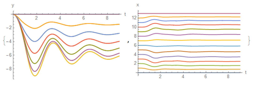
{Plot[Y, {t, 0, t0}, PlotRange -> All, AxesLabel -> {"t", "y"}], 
 Plot[X, {t, 0, t0}, PlotRange -> All, AxesLabel -> {"t", "x"}]}

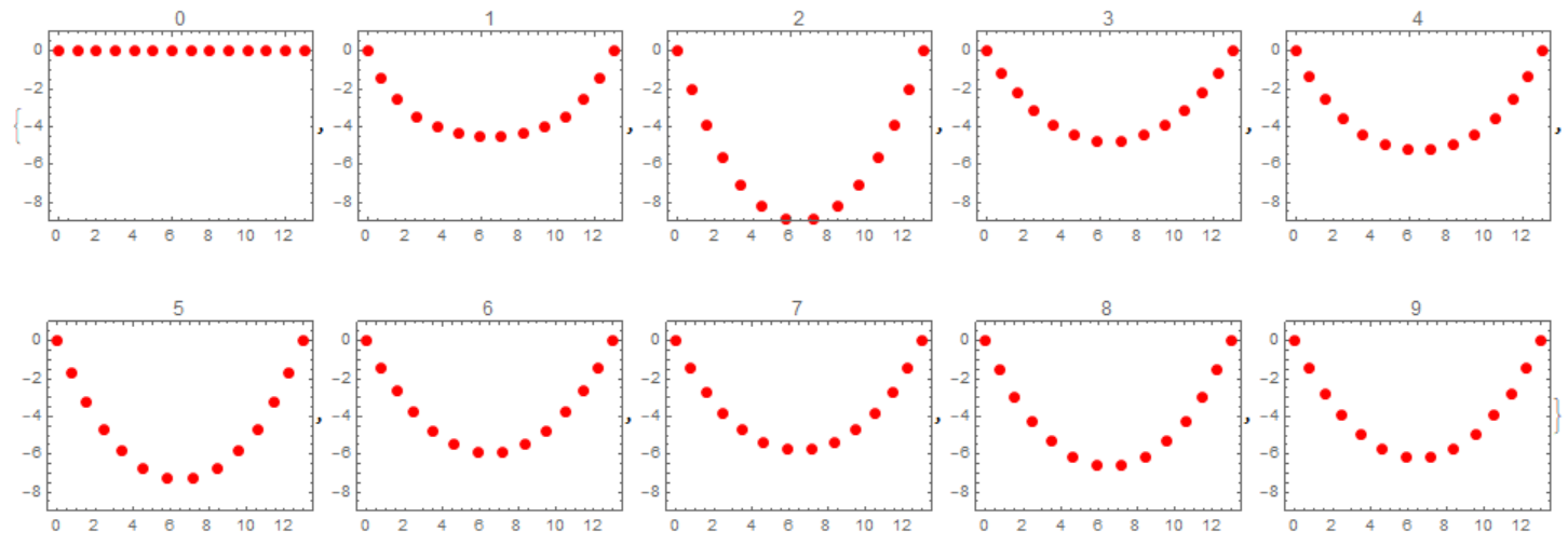
This figure shows the coordinates of the point masses. These coordinates can be displayed on the plane.

Table[Graphics[{PointSize[Large], Red, 
   Point[NDSolveValue[{eqns, ic, bc}, 
     Table[{x[i][tn], y[i][tn]}, {i, 1, P}], {t, 0, tn}]]}, 
  Frame -> True, PlotLabel -> tn, 
  PlotRange -> {{-.5, 13.5}, {-9, 1}}], {tn, 0, t0, 1}]

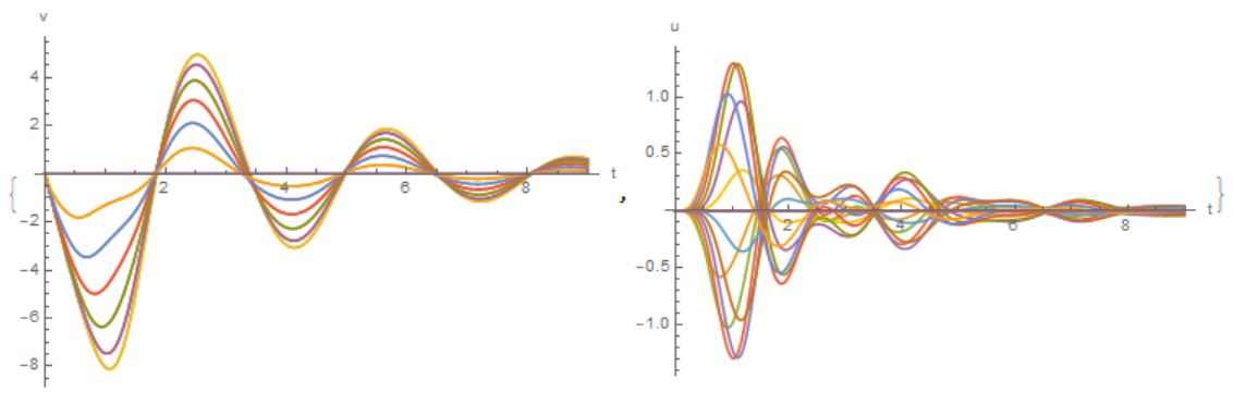
Velocity components of point masses

VY = NDSolveValue[{eqns, ic, bc}, 
  Table[y[i]'[t], {i, 1, P}], {t, 0, t0}]; VX = 
 NDSolveValue[{eqns, ic, bc}, Table[x[i]'[t], {i, 1, P}], {t, 0, t0}];
{Plot[VY, {t, 0, t0}, PlotRange -> All, AxesLabel -> {"t", "v"}], 
 Plot[VX, {t, 0, t0}, PlotRange -> All, AxesLabel -> {"t", "u"}]}

You can use any boundary conditions. This code is adapted for your task. However, you can use the code to solve a problem with one or two free ends. Therefore, accelerations are used as boundary conditions. An example of solving a problem with one free end

Thanks for the simplification. I understood the need for the simplification and can represent the acceleration and velocity as pure y''[t] and y'[t] due to symmetry but the position is needed to find the extension in the spring. I cant figure out another way to solve the extension in the spring.

You should post your code using the code sample icon (the first one).